---
title: "6 · End-to-end Parkfield walkthrough"
subtitle: "Phases 0–6 in a single `run_workflow` call"
jupyter: codameter-pixi
---
::: {.keyidea}
[Step goal]{.k-title}
Run the entire six-phase pipeline in one call and read the per-phase summary,
the diagnostic figure, and the posterior-predictive whiteness check that closes
the [Bayesian loop](theory-uq.qmd). This is the page to copy when you bring your
own data.
:::
```{python}
#| label: run
import sys, numpy as np, matplotlib.pyplot as plt
sys.path.insert(0, ".")
from _synth import make_synthetic, build_parkfield_site, set_style, C
from codameter import run_workflow
set_style()

dvv, forcings, eq_times, truth, comp = make_synthetic()
site = build_parkfield_site()
result = run_workflow(dvv, forcings, site, earthquake_times=eq_times)
print(result.summary())
```
## The six-panel diagnostic
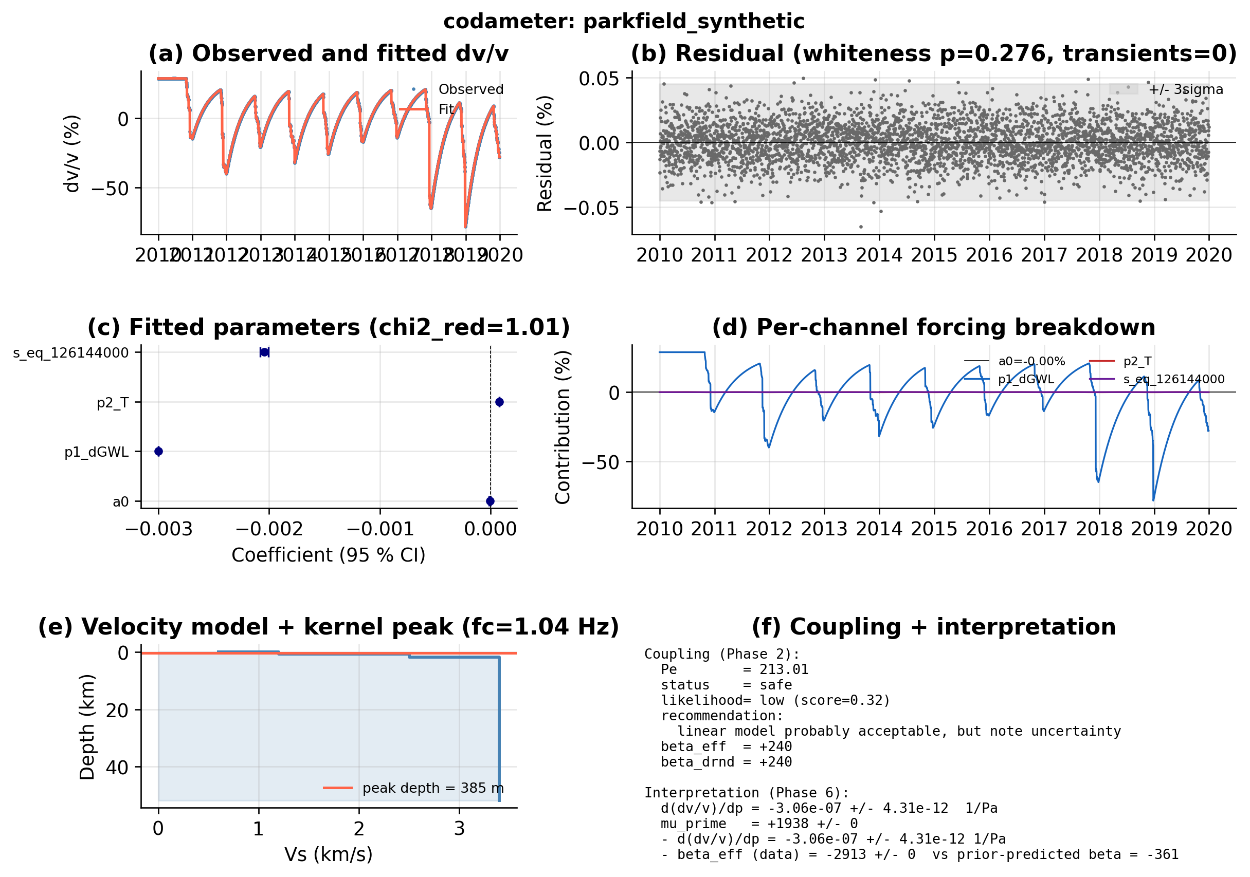
`result.plot_phases()` renders the canonical diagnostic the package ships — data,
fit, residuals, and phase summaries in one figure.
```{python}
#| label: fig-phases
#| fig-cap: "The codameter six-panel diagnostic for the synthetic Parkfield run, generated live by `result.plot_phases()`."
fig = result.plot_phases()
fig.set_size_inches(10, 7)
plt.show()
```
## Closing the loop with a posterior predictive check
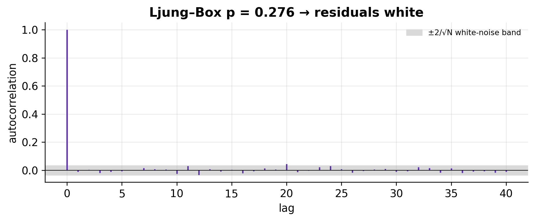
Phase 5 runs the Ljung–Box whiteness test ([Ljung–Box](theory-uq.qmd#eq-ljungbox)) on the standardised
residuals. A large $p$-value means the residuals are white — no evidence of
unmodelled physics — and the decoupled model is adequate. A small one would send
us back up the [iterative loop](theory-uq.qmd) to re-examine coupling or the
velocity model.
```{python}
#| label: ppc
a = result.phase5.report
print(f"Ljung–Box Q          : {a.whiteness_q:.2f}  ({a.whiteness_lags} lags)")
print(f"whiteness p-value    : {a.whiteness_pvalue:.3f}")
print(f"passes whiteness?    : {a.passes_whiteness}")
print(f"transients detected  : {a.n_transients}")
print(f"residual std         : {a.residual_std:.2e}")
```
```{python}
#| label: fig-ppc
#| fig-cap: "Residual autocorrelation. Bars inside the ±2/√N band (grey) are consistent with white noise — the posterior predictive check passes, so the linear-Gaussian inference stands for this site."
resid = result.phase4.fit.residuals
r = np.asarray(resid)
r = r[np.isfinite(r)]
r = r - r.mean()
nlags = 40
ac = np.array([1.0] + [np.corrcoef(r[:-k], r[k:])[0, 1] for k in range(1, nlags+1)])
band = 2.0 / np.sqrt(len(r))
fig, ax = plt.subplots(figsize=(9, 3))
ax.axhspan(-band, band, color="0.85", label="±2/√N white-noise band")
ax.vlines(range(len(ac)), 0, ac, color=C["accent"], lw=1.5)
ax.axhline(0, color="k", lw=0.6)
ax.set(xlabel="lag", ylabel="autocorrelation",
       title=f"Ljung–Box p = {a.whiteness_pvalue:.3f} → residuals white")
ax.legend(fontsize=8, frameon=False)
plt.show()
```
## Bringing your own data
The exact same call works on real data — supply a `dvv` DataFrame (with a
`dvv_err` column), a forcings dict, and a `Site` from your YAML:
```python
from codameter import run_workflow, load_site
from codameter.data import load_dvv, load_timeseries

site = load_site("examples/configs/parkfield.yaml")
dvv  = load_dvv("my_dvv.parquet")          # needs columns dvv, dvv_err
forc = {
    "temperature":   load_timeseries("T.csv"),
    "precipitation": load_timeseries("P.csv"),
}
result = run_workflow(dvv, forc, site)
result.export("runs/my_site/")             # summary, JSON, params, residuals, figure
```
Run `codameter data-check` first (see [step 1](tutorial-01-data.qmd)) to learn
what your file can honestly support.
---
::: {.keyidea}
[The whole arc, in one sentence]{.k-title}
We started from **completely decoupled** forward models, assembled them into a
linear-superposition inversion with an **exact Gaussian posterior**, used the
**coupling diagnostics** to decide that posterior is trustworthy here (and to
know when it would not be), and **propagated** it through the bridge relation to
stress and water-table change — *with intervals at every step.* That closed,
uncertainty-aware loop is the [contribution](theory-uq.qmd).
:::