---
title: "2 · Decoupled forward models"
subtitle: "Each stress source, modelled as if it acted alone"
jupyter: codameter-pixi
---
::: {.keyidea}
[Step goal]{.k-title}
This is the **"completely decoupled"** end of the arc. We treat the
thermoelastic, hydrological, and damage contributions as three independent
forward operators, each mapping one environmental driver to its own $\delta v/v$
footprint. Their *sum* is the linear-superposition model of [Eq. 6](theory-uq.qmd#eq-superpose).
:::
The decoupled assumption is the working hypothesis of most dv/v studies, and
for good reason: when it holds, the inverse problem is linear and the posterior
is exact and closed-form ([the Gaussian posterior](theory-uq.qmd#eq-gauss-post)). The job of this page is to *see* the
three footprints separately before we add them.
```{python}
#| label: setup
import sys, numpy as np, matplotlib.pyplot as plt
sys.path.insert(0, ".")
from _synth import make_synthetic, set_style, C, YEAR_S
from codameter.forward.thermoelastic import thermoelastic_dvv
from codameter.forward.poroelastic import baseflow_recharge_response
from codameter.forward.damage import snieder_healing
set_style()
dvv, forcings, eq_times, truth, comp = make_synthetic()
t = comp["times"]
```
## ① Thermoelastic — Berger / Okubo phase-shift
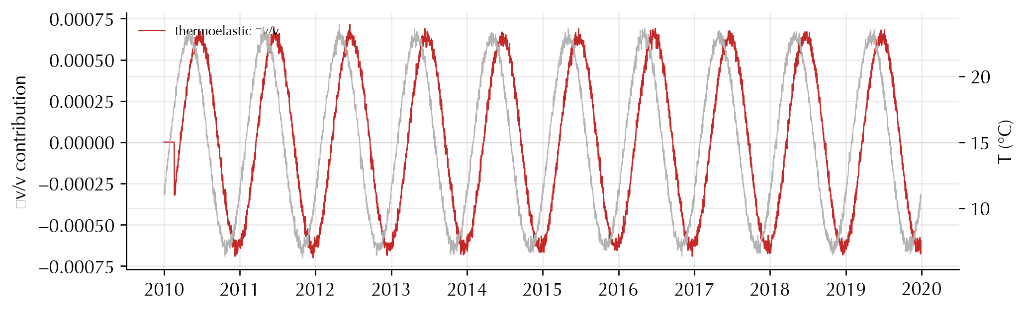
Surface temperature diffuses downward, and the thermal strain it induces at the
sensing depth lags the surface by a **phase shift** $t_{\text{shift}}$ (here 50
days). The forward model `thermoelastic_dvv` implements the @Okubo2024
phase-shift form [@Berger1975; @Okubo2024].
```{python}
#| label: fig-thermo
#| fig-cap: "Thermoelastic footprint. The δv/v response (red) is a phase-shifted, scaled copy of surface temperature (grey) — the 50-day lag is the downward thermal-diffusion delay."
t_s = (t - t[0]).total_seconds().to_numpy()
T_pred = thermoelastic_dvv(comp["T"], t_s, sensitivity_amplitude=1.0,
                           time_shift_days=50.0)
fig, ax = plt.subplots(figsize=(9, 2.8))
ax2 = ax.twinx()
ax2.plot(t, comp["T"], color="0.7", lw=0.6, label="surface T")
ax.plot(t, truth["p2_T"] * T_pred, color=C["thermo"], lw=0.8, label="thermoelastic δv/v")
ax.set(ylabel="δv/v contribution"); ax2.set(ylabel="T (°C)")
ax.legend(loc="upper left", fontsize=8, frameon=False)
plt.show()
```
## ② Hydrological — baseflow recharge proxy
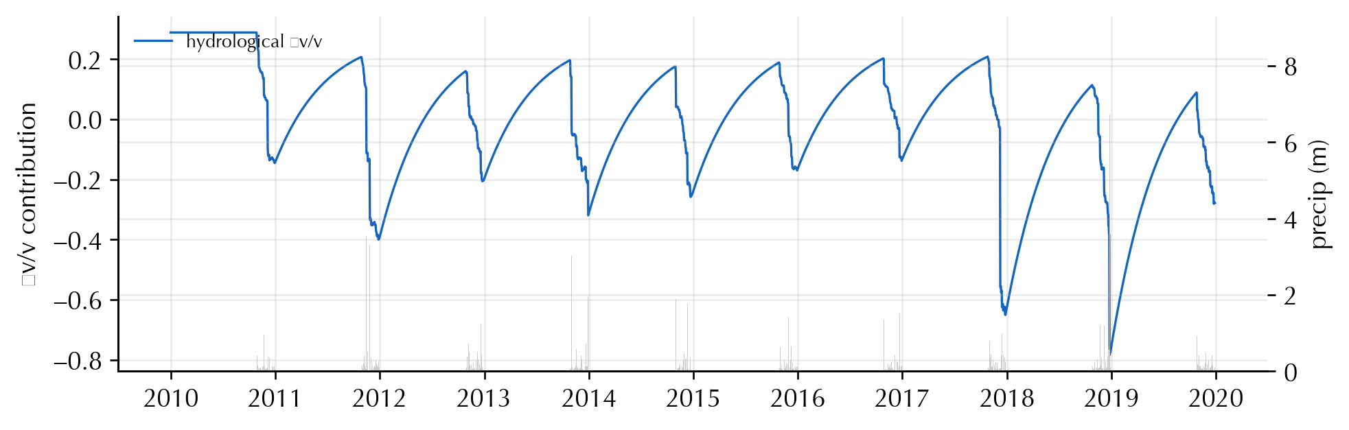
Precipitation recharges groundwater, and the rising water table changes pore
pressure and hence velocity. `baseflow_recharge_response` integrates sparse
storms into a slowly varying groundwater-level proxy $\Delta\mathrm{GWL}(t)$
[@Roeloffs1988; @Talwani2007]. Note the **sign**: more water → lower velocity.
```{python}
#| label: fig-hydro
#| fig-cap: "Hydrological footprint. Sparse winter storms (blue bars) integrate into a smooth seasonal-to-interannual groundwater signal (blue line). This is the term that becomes water-table depth in Phase 6."
dGWL = baseflow_recharge_response(comp["P"], t_s, porosity=0.05,
                                  decay_rate_per_s=1.0/(180*86400.0))
dGWL_c = dGWL - dGWL.mean()
fig, ax = plt.subplots(figsize=(9, 2.8))
ax2 = ax.twinx()
ax2.bar(t, comp["P"], color="0.8", width=2.0)
ax.plot(t, truth["p1_dGWL"] * dGWL_c, color=C["hydro"], lw=1.0, label="hydrological δv/v")
ax.set(ylabel="δv/v contribution"); ax2.set(ylabel="precip (m)")
ax.legend(loc="upper left", fontsize=8, frameon=False)
plt.show()
```
## ③ Damage & healing — Snieder logarithmic recovery
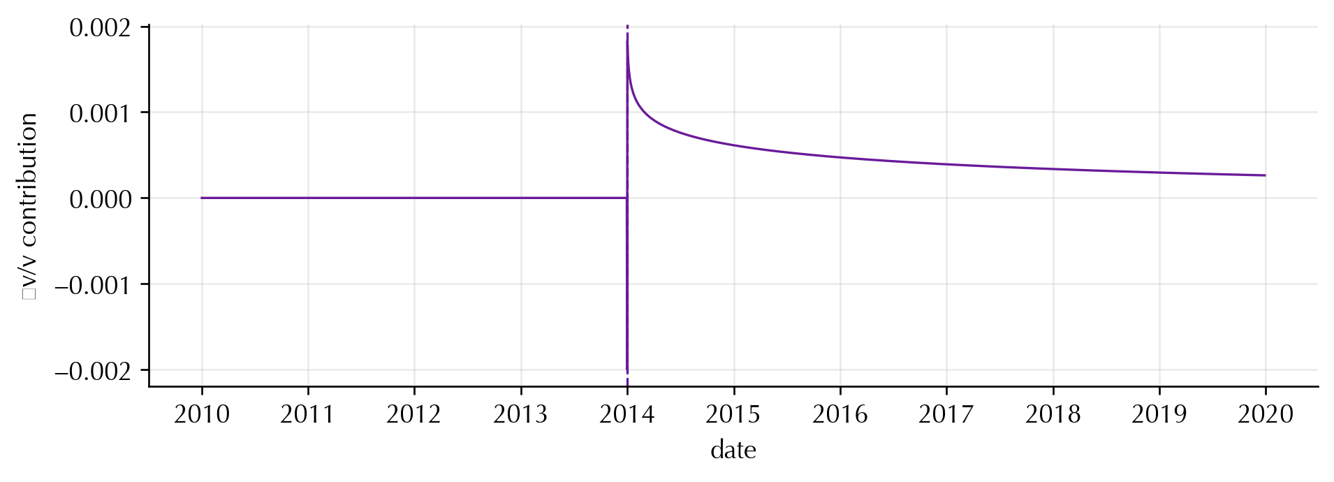
An earthquake drops the velocity abruptly (co-seismic damage) and the medium
then **heals logarithmically** in time. `snieder_healing` implements the
$\log(t/\tau)$ recovery between relaxation times $\tau_{\min}$ and $\tau_{\max}$
[@Snieder2017]. This is the term whose *time-dependence* will, in the coupled
regime, feed back on permeability.
```{python}
#| label: fig-damage
#| fig-cap: "Damage footprint. A co-seismic velocity drop at the 2014 event followed by logarithmic healing — the transient that anomaly detection (Phase 5) must not mistake for unmodelled physics."
eq_t_s = float((comp["eq_time"] - t[0]).total_seconds())
healing = snieder_healing(t_s - eq_t_s, tau_min_s=86400.0, tau_max_s=30*YEAR_S)
L0 = -np.log(30*YEAR_S/86400.0)
fig, ax = plt.subplots(figsize=(9, 2.8))
ax.plot(t, truth["s_eq"] * healing/L0, color=C["damage"], lw=1.0)
ax.axvline(comp["eq_time"], color=C["damage"], ls="--", lw=1.0)
ax.set(ylabel="δv/v contribution", xlabel="date")
plt.show()
```
## Superposition: the decoupled model
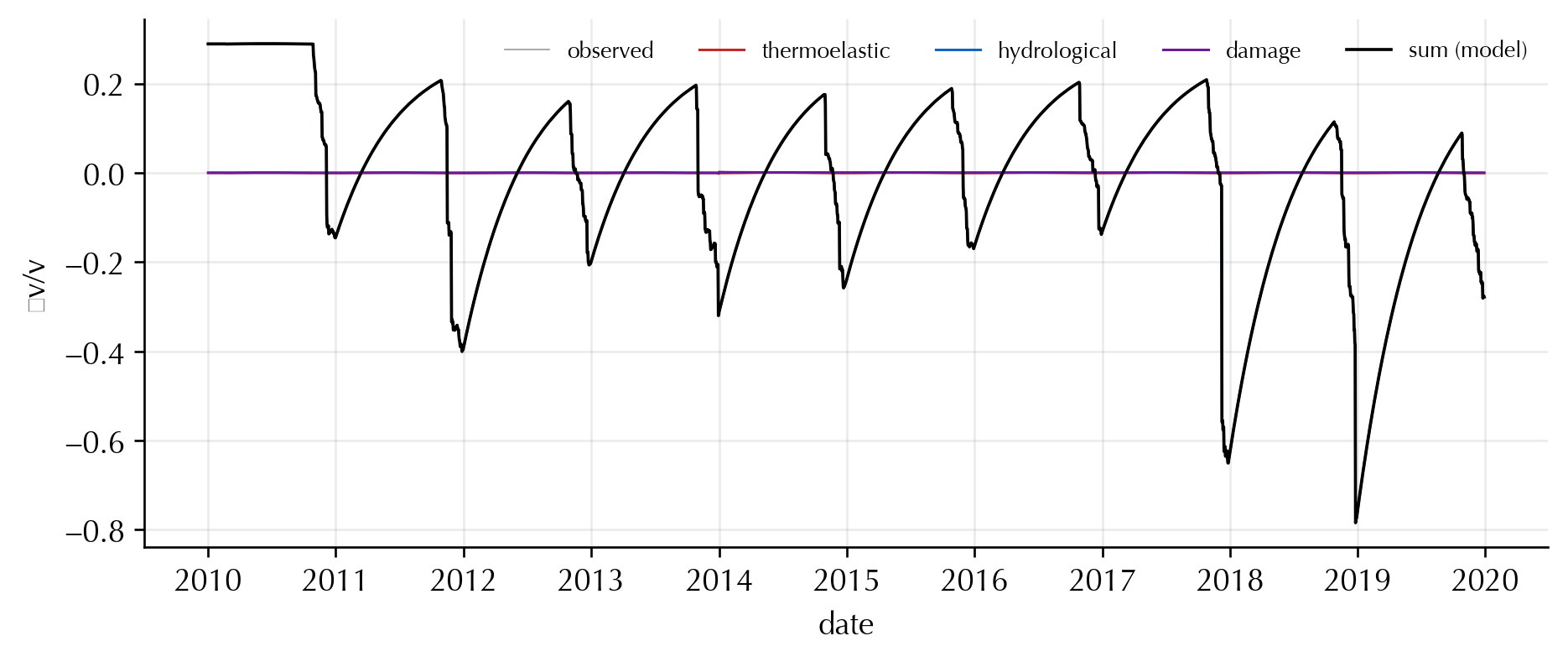
Under the decoupled hypothesis, the observed $\delta v/v$ is just the **sum** of
the three footprints plus noise. This stacked view is the visual statement of
[Eq. 6](theory-uq.qmd#eq-superpose) — and the assumption the next two pages will test and, eventually,
break.
```{python}
#| label: fig-stack
#| fig-cap: "The decoupled decomposition. Three independent forward models stack to reproduce the observed series. Step 3 inverts this picture; step 4 asks when the 'independent' assumption fails."
fig, ax = plt.subplots(figsize=(9, 3.4))
ax.plot(t, dvv.dvv, color="0.6", lw=0.5, label="observed")
ax.plot(t, comp["thermo"], color=C["thermo"], lw=0.9, label="thermoelastic")
ax.plot(t, comp["hydro"],  color=C["hydro"],  lw=0.9, label="hydrological")
ax.plot(t, comp["damage"], color=C["damage"], lw=0.9, label="damage")
ax.plot(t, comp["clean"],  color="k", lw=1.1, label="sum (model)")
ax.set(ylabel="δv/v", xlabel="date")
ax.legend(loc="upper right", ncol=5, fontsize=8, frameon=False)
plt.show()
```
→ Next: [Linear superposition & inversion](tutorial-03-inversion.qmd) — recover
the amplitudes *and their covariance* from the data.
### References {.unnumbered}
::: {#refs}
:::