1 · Data & site readiness

Phases 0–1 — what your data can honestly support

Step goal Before any physics, answer two questions: (i) is the $\delta v/v$ series clean and does it carry a measurement uncertainty? and (ii) at what depth does this measurement actually sense stress? Both feed everything downstream — including the uncertainty budget.

We work the whole tutorial on a synthetic Parkfield dataset so every figure is reproducible with no downloads. The generator forward-models a thermoelastic term, a hydrological (groundwater) term, and an earthquake-healing term, then adds Gaussian noise — it is the same construction as examples/01_parkfield_synthetic.py.

Code

import sys, numpy as np, pandas as pd, matplotlib.pyplot as plt
sys.path.insert(0, ".")
from _synth import make_synthetic, build_parkfield_site, set_style, C
set_style()

dvv, forcings, eq_times, truth, comp = make_synthetic()
site = build_parkfield_site()
dvv.head()

	dvv	dvv_err
2010-01-01 00:00:00+00:00	0.288690	0.00015
2010-01-02 00:00:00+00:00	0.288521	0.00015
2010-01-03 00:00:00+00:00	0.288627	0.00015
2010-01-04 00:00:00+00:00	0.288949	0.00015
2010-01-05 00:00:00+00:00	0.288768	0.00015

The observation and its uncertainty

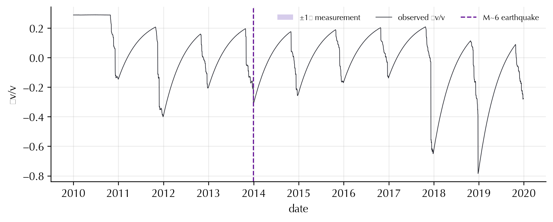
The single most important column — and the one most datasets omit — is dvv_err. Without it there is no principled weighting in the inversion and no posterior: the entire Bayesian story starts from the per-sample $\sigma_t$ in the likelihood. Here it is a constant $1.5\times10^{-4}$.

Code

fig, ax = plt.subplots(figsize=(9, 3.2))
t = dvv.index
ax.fill_between(t, dvv.dvv - dvv.dvv_err, dvv.dvv + dvv.dvv_err,
                color=C["band"], alpha=0.25, lw=0, label="±1σ measurement")
ax.plot(t, dvv.dvv, color=C["dvv"], lw=0.6, label="observed δv/v")
ax.axvline(comp["eq_time"], color=C["damage"], ls="--", lw=1.2, label="M~6 earthquake")
ax.set(ylabel="δv/v", xlabel="date")
ax.legend(loc="upper right", ncol=3, fontsize=8, frameon=False)
plt.show()

Figure 1: Ten years of synthetic δv/v with its ±1σ measurement band. The seasonal swing is the superposition of (still-hidden) thermoelastic and hydrological forcings; the step near 2014 is the earthquake.

What is driving it? The raw forcings

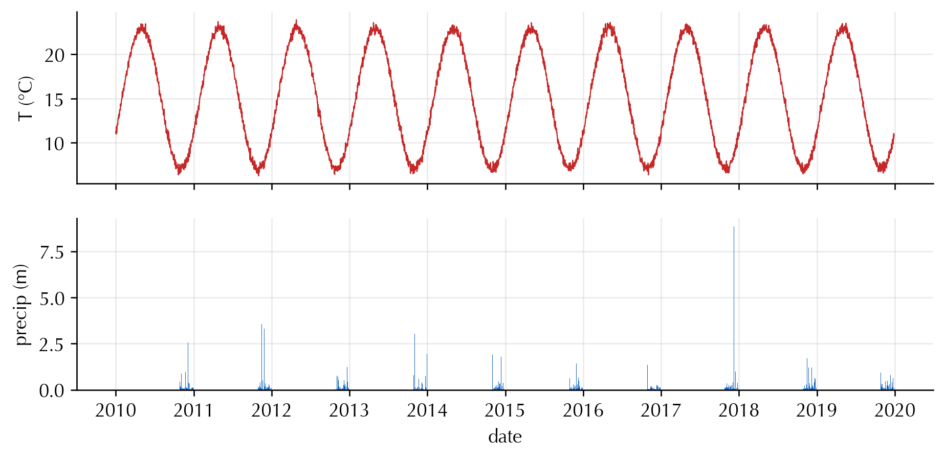
Two environmental series accompany the $\delta v/v$: surface temperature and precipitation. In the next step we turn each into a predicted $\delta v/v$ footprint; for now we just look at the drivers.

Code

fig, axes = plt.subplots(2, 1, figsize=(9, 4), sharex=True)
axes[0].plot(forcings["temperature"].index, forcings["temperature"].values,
             color=C["thermo"], lw=0.7)
axes[0].set(ylabel="T (°C)")
axes[1].bar(forcings["precipitation"].index, forcings["precipitation"].values,
            color=C["hydro"], width=2.0)
axes[1].set(ylabel="precip (m)", xlabel="date")
plt.show()

Figure 2: The raw environmental forcings. Temperature is a clean seasonal cycle; precipitation is sparse winter storms whose recharge integrates into a slow groundwater signal.

Phase 1 — at what depth are we sensing?

A $\delta v/v$ measured in a frequency band does not sense a point; it senses a depth kernel. Phase 1 either computes the Rayleigh-wave sensitivity kernel (if disba is installed) or falls back to the $z_{\text{peak}}\approx V_S/3f$ rule of thumb (Hillers et al. 2015). The peak depth sets where the stress estimate in step 5 applies, and the elastic moduli at that depth enter the bridge relation the bridge chain.

Code

from codameter import Phase1
p1 = Phase1.run(site)
print(f"central frequency : {p1.central_frequency_hz:.3f} Hz")
print(f"peak depth        : {p1.peak_depth_km*1e3:.0f} m")
print(f"shear modulus  μ  : {p1.shear_modulus_pa_at_peak/1e9:.2f} GPa")
print(f"bulk modulus   κ  : {p1.bulk_modulus_pa_at_peak/1e9:.2f} GPa")
p1.depth_table

central frequency : 1.039 Hz
peak depth        : 385 m
shear modulus  μ  : 3.17 GPa
bulk modulus   κ  : 9.53 GPa

	frequency_hz	peak_depth_km	half_max_top_km	half_max_bottom_km	vs_at_peak	rho_at_peak	mu_at_peak_GPa
0	1.03923	0.3849	0.19245	0.57735	1.2	2.2	3.168

Carry-forward We now know the measurement senses ~385 m depth, with moduli that we will need — with their prior uncertainty — to convert a fitted regression coefficient into stress. The depth and moduli are deterministic here, but the moduli priors are where a large share of the final stress uncertainty will come from.

Readiness gate

codameter ships a data-check that converts all of this into a go / no-go report per scientific goal (groundwater, stress, coupling). The rule it encodes is blunt and worth repeating: precipitation + δv/v supports a relative storage proxy; absolute groundwater or stress needs independent calibration. That honesty about what the data cannot support is the same instinct that motivates the Bayesian uncertainty treatment.

→ Next: Decoupled forward models — turning each forcing into a predicted $\delta v/v$.

References

Hillers, Gregor, Stephan Husen, Anne Obermann, Thomas Planès, Eric Larose, and Michel Campillo. 2015. “Noise-Based Monitoring and Imaging of Aseismic Transient Deformation Induced by the 2006 Basel Reservoir Stimulation.” Geophysics 80: KS51–68. https://doi.org/10.1190/geo2014-0455.1.

--- title: "1 · Data & site readiness" subtitle: "Phases 0–1 — what your data can honestly support" jupyter: codameter-pixi --- ::: {.keyidea} [Step goal]{.k-title} Before any physics, answer two questions: *(i)* is the $\delta v/v$ series clean and does it carry a measurement uncertainty? and *(ii)* at what **depth** does this measurement actually sense stress? Both feed everything downstream — including the uncertainty budget. ::: We work the whole tutorial on a **synthetic Parkfield** dataset so every figure is reproducible with no downloads. The generator forward-models a thermoelastic term, a hydrological (groundwater) term, and an earthquake-healing term, then adds Gaussian noise — it is the same construction as `examples/01_parkfield_synthetic.py`. ```{python} #| label: setup import sys, numpy as np, pandas as pd, matplotlib.pyplot as plt sys.path.insert(0, ".") from _synth import make_synthetic, build_parkfield_site, set_style, C set_style() dvv, forcings, eq_times, truth, comp = make_synthetic() site = build_parkfield_site() dvv.head() ``` ## The observation and its uncertainty The single most important column — and the one most datasets omit — is `dvv_err`. Without it there is no principled weighting in the inversion and **no posterior**: the entire [Bayesian story](theory-uq.qmd) starts from the per-sample $\sigma_t$ in [the likelihood](theory-uq.qmd#eq-like). Here it is a constant $1.5\times10^{-4}$. ```{python} #| label: fig-obs #| fig-cap: "Ten years of synthetic δv/v with its ±1σ measurement band. The seasonal swing is the superposition of (still-hidden) thermoelastic and hydrological forcings; the step near 2014 is the earthquake." fig, ax = plt.subplots(figsize=(9, 3.2)) t = dvv.index ax.fill_between(t, dvv.dvv - dvv.dvv_err, dvv.dvv + dvv.dvv_err, color=C["band"], alpha=0.25, lw=0, label="±1σ measurement") ax.plot(t, dvv.dvv, color=C["dvv"], lw=0.6, label="observed δv/v") ax.axvline(comp["eq_time"], color=C["damage"], ls="--", lw=1.2, label="M~6 earthquake") ax.set(ylabel="δv/v", xlabel="date") ax.legend(loc="upper right", ncol=3, fontsize=8, frameon=False) plt.show() ``` ## What is driving it? The raw forcings Two environmental series accompany the $\delta v/v$: surface temperature and precipitation. In the [next step](tutorial-02-forward.qmd) we turn each into a *predicted* $\delta v/v$ footprint; for now we just look at the drivers. ```{python} #| label: fig-forcings #| fig-cap: "The raw environmental forcings. Temperature is a clean seasonal cycle; precipitation is sparse winter storms whose recharge integrates into a slow groundwater signal." fig, axes = plt.subplots(2, 1, figsize=(9, 4), sharex=True) axes[0].plot(forcings["temperature"].index, forcings["temperature"].values, color=C["thermo"], lw=0.7) axes[0].set(ylabel="T (°C)") axes[1].bar(forcings["precipitation"].index, forcings["precipitation"].values, color=C["hydro"], width=2.0) axes[1].set(ylabel="precip (m)", xlabel="date") plt.show() ``` ## Phase 1 — at what depth are we sensing? A $\delta v/v$ measured in a frequency band does not sense a point; it senses a **depth kernel**. Phase 1 either computes the Rayleigh-wave sensitivity kernel (if `disba` is installed) or falls back to the $z_{\text{peak}}\approx V_S/3f$ rule of thumb [@Hillers2015]. The peak depth sets *where* the stress estimate in [step 5](tutorial-05-interpretation.qmd) applies, and the elastic moduli at that depth enter the bridge relation [the bridge chain](theory-uq.qmd#eq-chain). ```{python} #| label: phase1 from codameter import Phase1 p1 = Phase1.run(site) print(f"central frequency : {p1.central_frequency_hz:.3f} Hz") print(f"peak depth : {p1.peak_depth_km*1e3:.0f} m") print(f"shear modulus μ : {p1.shear_modulus_pa_at_peak/1e9:.2f} GPa") print(f"bulk modulus κ : {p1.bulk_modulus_pa_at_peak/1e9:.2f} GPa") p1.depth_table ``` ::: {.keyidea} [Carry-forward]{.k-title} We now know the measurement senses **~385 m depth**, with moduli that we will need — *with their prior uncertainty* — to convert a fitted regression coefficient into stress. The depth and moduli are deterministic here, but the *moduli priors* are where a large share of the final stress uncertainty will come from. ::: ## Readiness gate `codameter` ships a `data-check` that converts all of this into a go / no-go report per scientific goal (groundwater, stress, coupling). The rule it encodes is blunt and worth repeating: **precipitation + δv/v supports a *relative* storage proxy; absolute groundwater or stress needs independent calibration.** That honesty about what the data cannot support is the same instinct that motivates the [Bayesian uncertainty treatment](theory-uq.qmd). → Next: [Decoupled forward models](tutorial-02-forward.qmd) — turning each forcing into a predicted $\delta v/v$. ### References {.unnumbered} ::: {#refs} :::