---
title: "5 · Interpreting stress at depth"
subtitle: "Phase 6 — pushing the posterior through the bridge relation"
jupyter: codameter-pixi
---
::: {.keyidea}
[Step goal]{.k-title}
This is where the Bayesian framing pays its rent. The fitted hydrological
coefficient $p_1$ is **not** stress; stress is a *derived* quantity reached by
chaining three transformations ([the bridge chain](theory-uq.qmd#eq-chain)), each involving an uncertain
material parameter. We propagate the posterior all the way through and report
stress sensitivity **with an interval**.
:::
```{python}
#| label: setup
import sys, numpy as np, matplotlib.pyplot as plt
sys.path.insert(0, ".")
from _synth import make_synthetic, build_parkfield_site, set_style, C
from codameter import run_workflow
set_style()
dvv, forcings, eq_times, truth, comp = make_synthetic()
site = build_parkfield_site()
result = run_workflow(dvv, forcings, site, earthquake_times=eq_times)
p6 = result.phase6
```
## The propagation chain
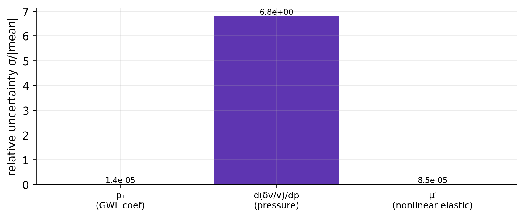
Phase 6 takes $p_1$ (fraction per metre of head), divides by $\rho g$ to get a
**pressure sensitivity** $d(\delta v/v)/dp$, multiplies by the bulk modulus to
get an **effective acoustoelastic** $\beta_{\text{eff}}$, and finally inverts the
**bridge relation** $\beta=-\mu'\kappa/2\mu$ to estimate $\mu'$. Every step
carries an uncertainty forward via the delta method ([the delta method](theory-uq.qmd#eq-delta)).
```{python}
#| label: chain
ps_mean, ps_var = p6.pressure_sensitivity
mp_mean, mp_var = p6.mu_prime_estimate
print(f"pressure sensitivity d(δv/v)/dp : {ps_mean:.3e} ± {np.sqrt(ps_var):.2e} 1/Pa")
print(f"μ′ estimate                     : {mp_mean:.1f} ± {np.sqrt(mp_var):.2f}")
for n in p6.notes:
    print(" •", n)
```
```{python}
#| label: fig-chain
#| fig-cap: "The interpretation chain as an uncertainty pipeline. A coefficient with a tight relative error (left) inherits the *material-property* uncertainty at each transform — the final stress-relevant quantity's error budget is dominated not by measurement noise but by the priors on ρ, κ, μ."
fit = result.phase4.fit
p1_m, p1_s = fit.posterior.marginal("p1_dGWL")
stages = ["p₁\n(GWL coef)", "d(δv/v)/dp\n(pressure)", "μ′\n(nonlinear elastic)"]
means = [abs(p1_m), abs(ps_mean), mp_mean]
rel   = [p1_s/abs(p1_m), np.sqrt(ps_var)/abs(ps_mean), np.sqrt(mp_var)/mp_mean]
fig, ax = plt.subplots(figsize=(7.5, 3.2))
xs = range(len(stages))
ax.bar(xs, rel, color=[C["hydro"], C["band"], C["thermo"]])
ax.set_xticks(list(xs)); ax.set_xticklabels(stages, fontsize=9)
ax.set(ylabel="relative uncertainty σ/|mean|")
for x, r in zip(xs, rel):
    ax.text(x, r, f"{r:.1e}", ha="center", va="bottom", fontsize=8)
plt.tight_layout(); plt.show()
```
## Water-table change with its uncertainty band
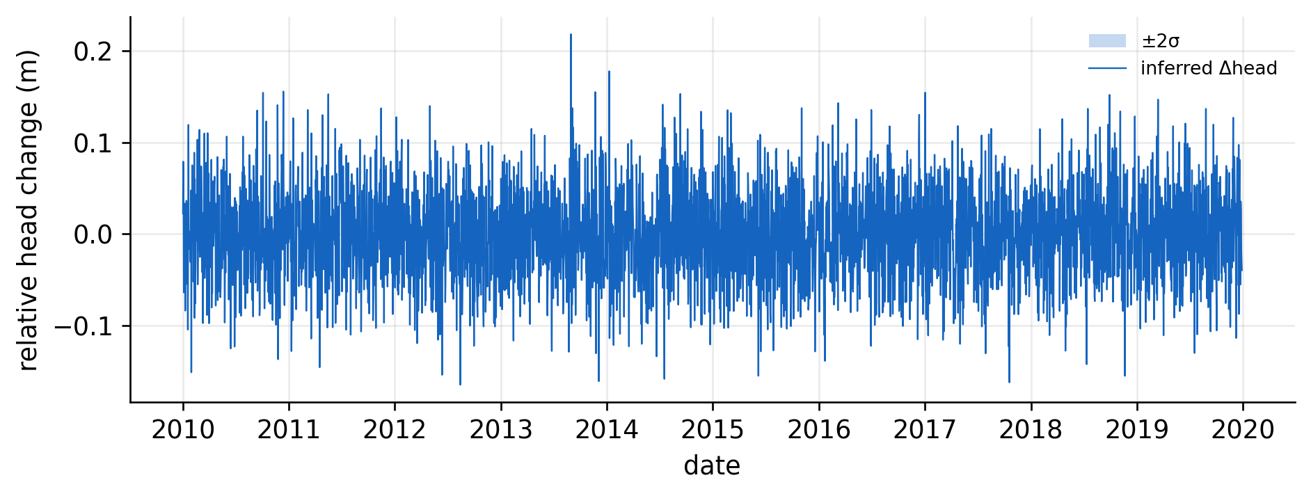
The same hydrological coefficient, read the other way, converts $\delta v/v$
into a relative **head change** time series — each sample carrying its own
propagated $\sigma$ (Phase 6's v0.1 scalar inversion; the full
saturation-aware, water-budget version is v0.2).
```{python}
#| label: fig-head
#| fig-cap: "Inferred relative water-table change with its ±2σ propagated band. The band is the pushforward of the posterior through the inversion — a per-sample uncertainty, not a single error bar."
wt = p6.head_change
h = np.asarray(wt.head_change_m)
hs = np.asarray(wt.head_change_std_m)
fig, ax = plt.subplots(figsize=(9, 3))
ax.fill_between(dvv.index, h-2*hs, h+2*hs, color=C["hydro"], alpha=0.25,
                lw=0, label="±2σ")
ax.plot(dvv.index, h, color=C["hydro"], lw=0.7, label="inferred Δhead")
ax.set(ylabel="relative head change (m)", xlabel="date")
ax.legend(fontsize=8, frameon=False, loc="upper right")
plt.show()
```
## Why a Monte-Carlo pushforward, not just the delta method
The delta method ([the delta method](theory-uq.qmd#eq-delta)) is exact only when the transform is linear and the
posterior Gaussian. The bridge relation involves a **product** of uncertain
moduli, so for a fully honest interval — especially once the
[coupled regime](tutorial-04-coupling.qmd) makes the posterior non-Gaussian — we
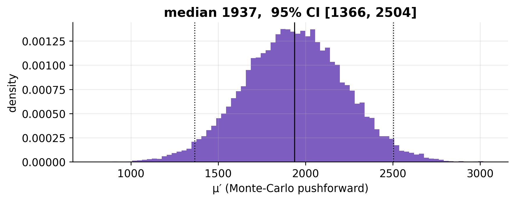
draw samples and push each through $g$. We illustrate with a Monte-Carlo
pushforward of $\mu'$ using the posterior on $p_1$ and prior uncertainty on the
moduli.
```{python}
#| label: fig-mc
#| fig-cap: "Monte-Carlo pushforward of μ′. Sampling p₁ from its posterior and the moduli from their priors, then evaluating the bridge relation per draw, yields the full derived distribution — the object the theory page argues should replace a point estimate."
rng = np.random.default_rng(0)
N = 20000
p1_draws = rng.normal(p1_m, p1_s, N)
# illustrative ±15% prior spread on the moduli entering the bridge relation
kappa = result.phase1.bulk_modulus_pa_at_peak * rng.normal(1.0, 0.15, N)
mu    = result.phase1.shear_modulus_pa_at_peak * rng.normal(1.0, 0.15, N)
rho_g = 1000.0 * 9.81
beta_eff = (p1_draws / rho_g) * kappa
mu_prime = -2.0 * mu / kappa * beta_eff
fig, ax = plt.subplots(figsize=(7.5, 3))
ax.hist(mu_prime, bins=80, color=C["band"], alpha=0.8, density=True)
q = np.percentile(mu_prime, [2.5, 50, 97.5])
for v, ls in zip(q, [":", "-", ":"]):
    ax.axvline(v, color="k", ls=ls, lw=1)
ax.set(xlabel="μ′ (Monte-Carlo pushforward)", ylabel="density",
       title=f"median {q[1]:.0f},  95% CI [{q[0]:.0f}, {q[2]:.0f}]")
plt.tight_layout(); plt.show()
```
::: {.callout-note}
The MC interval is **wider** than the delta-method one above because it folds in
the material-property prior uncertainty that the closed-form propagation around
the fitted coefficient alone does not see. That gap *is* the argument of the
[theory page](theory-uq.qmd): the dominant uncertainty in interpreted stress is
the priors, not the measurement noise.
:::
→ Next: [End-to-end Parkfield walkthrough](tutorial-06-endtoend.qmd) — the whole
pipeline in one run.