---
title: "δv/v → δVs(z)/Vs: propagating measurement error to depth"
subtitle: "Window rules as Bayesian nuisance parameters, carried into a depth inversion"
jupyter: codameter-pixi
bibliography: references.bib
---
::: {.keyidea}
[Thesis]{.k-title}
This is **step 2 of the uncertainty arc**. We have the within-method **floor**
and the **temporal correlation** from
[step 1 · measurement](theory-measurement-uq.qmd). This page closes the last two
gaps: *(i)* how to **sample** the uncertainty in the processing *choices
themselves* — window length, coda start, and especially the **rule** that defines
the window (fixed, envelope-pick-to-flattening, moving) — by treating them as
Bayesian **nuisance parameters** and marginalising them; and *(ii)* how to make
**one error per frequency band** and propagate those errors through a sensitivity
**kernel** into a **depth profile** of $\delta V_S/V_S(z)$ with an honest
uncertainty envelope — the covariance [step 3 · stress](uncertainty-3-stress.qmd)
consumes.
:::
### Where the field stands
The field has converged on one physical rule for depth — *depth is set by the
frequency band and the coda lapse time, not assumed* [@Obermann2013; @Obermann2016]
— and, increasingly, on multi-band measurement to resolve it [@Takano2017; @Feng2020; @Mao2022]. The step from per-band $\delta v/v$ to a depth
profile is where reporting is least consistent: many studies read one band as one
depth, only a few invert several bands against sensitivity kernels, and the
measurement error is seldom propagated into the depth estimate. The depth
assignment is frequently the scientific claim itself — whether the change lies in
the aquifer or the overlying soil [@Rubinstein2005] — so a depth reported
without its uncertainty cannot support that claim.
| Choice | Best practice | Common deviation | Consequence |
|---|---|---|---|
| Depth assignment | Invert several bands against sensitivity kernels | Read one band as one depth | No depth resolution or error |
| Band selection | Bands where the kernels resolve (no half-space leak, coherent coda) | Convenience band | Kernel leaks; unstable inversion |
| Measurement error | Propagate the per-band $C_d$ into the profile | Plot a profile with no covariance | Overconfident depth attribution |
| Saturation | Separate $\delta V_S/V_S$ and $\delta\rho/\rho$ with a petrophysical model | Assume a pure $\delta V_S/V_S$ change | Biased velocity change and stress in hydrological / cryospheric targets |
| Velocity model | State the reference $V_P,V_S(z)$ and its uncertainty | Fixed, unstated model | Hidden systematic in the kernels and moduli |
```{python}
#| label: setup
import sys, numpy as np, matplotlib.pyplot as plt
sys.path.insert(0, ".")
from _synth import build_parkfield_site, set_style, C
set_style()
from codameter.uq_processing import (
    ProcessingPrior, sample_processing_choices, per_band_marginal_error,
    flatten_end_lapse, choice_floor)
from codameter.uq_depth import band_sensitivity_matrix, invert_depth_profile
from codameter.kernels import make_fine_model
rng = np.random.default_rng(11)
```
## 1. The window *rule* is the deep, frequency-dependent choice
Different groups do not just pick different numbers; they pick different
*algorithms* for where the coda window goes. Three dominate:
| Rule | Start $t_1$ | End $t_2$ | Character |
|---|---|---|---|
| **fixed** | a habitual lapse | $t_1 + L$, fixed $L$ | simple, frequency-blind |
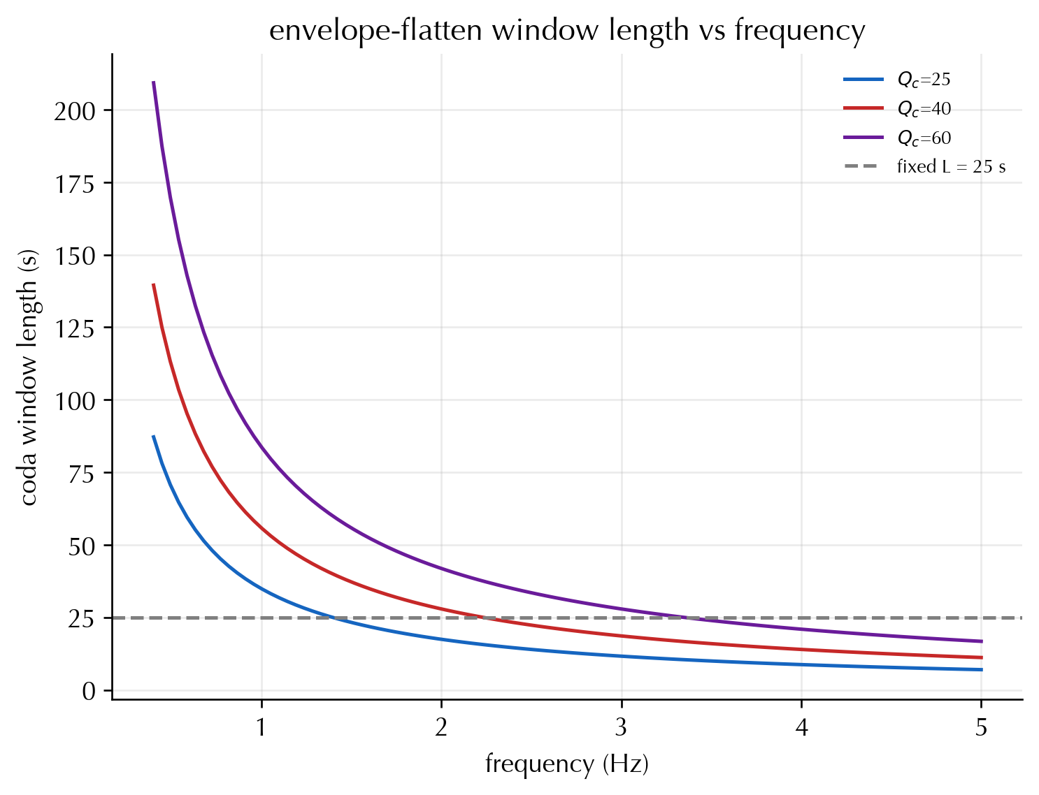
| **envelope pick → flatten** | the envelope **pick** | where $\log A(t)$ **flattens** into noise | *physical*, frequency-dependent |
| **moving** | slides along the coda | short window, many positions | samples a range of scattering depths |
The envelope rule is the interesting one. With coda decay
$A(t)\propto e^{-\pi f t/Q_c}$, the log-envelope flattens into the noise floor at
$$
t_2 = t_1 + \frac{Q_c}{\pi f}\,\ln(\mathrm{SNR}_0),
$$ {#eq-flatten}
so the window **shrinks as frequency rises** — exactly where a fixed window
silently disagrees. `flatten_end_lapse` encodes this.
```{python}
#| label: fig-rules
#| fig-cap: "The envelope-flatten rule (Eq. 1) makes the usable coda length frequency-dependent: high-frequency coda decays into the noise sooner, so its window is shorter. A fixed window (grey) ignores this — the two rules agree only near one frequency, and disagree everywhere else. That disagreement is a measurement uncertainty."
f = np.linspace(0.4, 5, 100)
for qc, col in [(25, C["hydro"]), (40, C["thermo"]), (60, C["damage"])]:
    ax_end = [flatten_end_lapse(8.0, fi, qc, 80) - 8.0 for fi in f]
    plt.plot(f, ax_end, color=col, label=f"$Q_c$={qc}")
plt.axhline(25, color="0.5", ls="--", label="fixed L = 25 s")
plt.xlabel("frequency (Hz)"); plt.ylabel("coda window length (s)")
plt.title("envelope-flatten window length vs frequency")
plt.legend(fontsize=8, frameon=False); plt.show()
```
## 2. Sampling the choices as a Bayesian "multiverse"
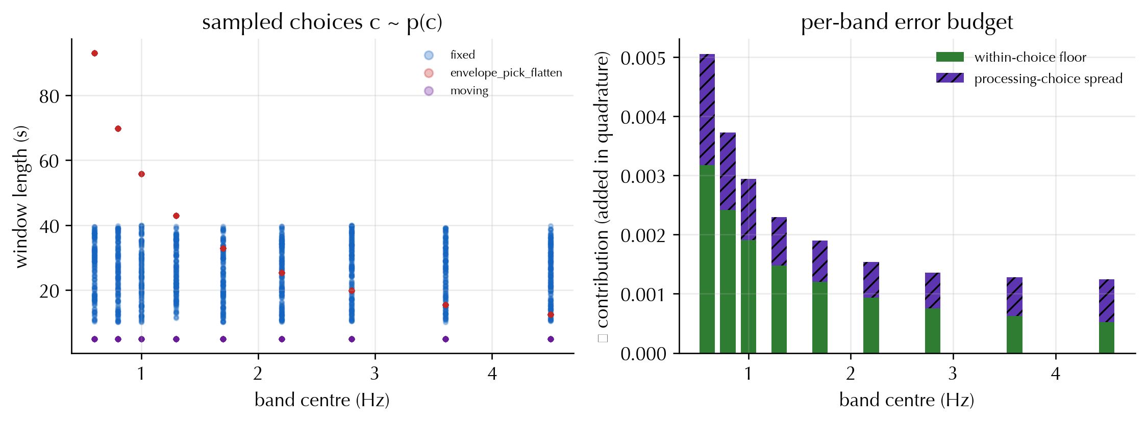
To be Bayesian about the choice, we put a prior $p(c)$ over the whole
configuration $c=(\text{rule}, t_1, L, f, \dots)$ and **sample** it — a Monte
Carlo over the analysis multiverse [@Steegen2016]. Each draw yields a coda
window and, through the Weaver/Clarke floor, a within-choice error. The law of
total variance then splits the marginal measurement variance into a
**within-choice floor** and a **processing-choice spread**:
$$
\operatorname{Var}(\delta v/v) =
\underbrace{\mathbb{E}_c[\operatorname{Var}(\delta v/v\mid c)]}_{\text{floor}}
+\underbrace{\operatorname{Var}_c[\mathbb{E}(\delta v/v\mid c)]}_{\text{choice spread}} .
$$ {#eq-ltv}
```{python}
#| label: sample
bands = np.array([0.6, 0.8, 1.0, 1.3, 1.7, 2.2, 2.8, 3.6, 4.5])
prior = ProcessingPrior(
    bands_hz=bands,
    rule_weights={"fixed": 0.5, "envelope_pick_flatten": 0.3, "moving": 0.2},
    start_lapse_s=(4.0, 12.0), window_length_s=(10.0, 40.0), qc=40.0, snr0=80.0,
)
choices = sample_processing_choices(prior, 12000, rng)
# a (illustrative) per-band methodological bias: estimators disagree more at
# high frequency where the windows are shortest and the codas least coherent.
band_bias = {float(f): 2.5e-4 + 1.0e-4 * f for f in bands}
pbe = per_band_marginal_error(choices, band_bias=band_bias)
for f in bands:
    s = pbe[float(f)]
    print(f"{f:>4.1f} Hz  floor={s['within']:.2e}  choice={s['processing']:.2e}  "
          f"total={s['total']:.2e}  (n={s['n']:.0f})")
```
```{python}
#| label: fig-multiverse
#| fig-cap: "Left: the sampled coda windows, coloured by rule — the envelope rule (red) sweeps a frequency-dependent locus, the moving rule (purple) scatters along the coda, the fixed rule (blue) clusters by habit. Right: the per-band error budget. The processing-choice spread (hatched) is a large, irreducible part of the total that no single pipeline reveals."
fig, ax = plt.subplots(1, 2, figsize=(9.5, 3.6), gridspec_kw={"width_ratios":[1.1,1]})
rule_col = {"fixed": C["hydro"], "envelope_pick_flatten": C["thermo"], "moving": C["damage"]}
for rule in rule_col:
    sub = [c for c in choices[:2500] if c.rule == rule]
    ax[0].scatter([c.f_center_hz for c in sub], [c.t2_s - c.t1_s for c in sub],
                  s=6, alpha=0.3, color=rule_col[rule], label=rule)
ax[0].set(xlabel="band centre (Hz)", ylabel="window length (s)",
          title="sampled choices c ~ p(c)")
ax[0].legend(fontsize=7, frameon=False, markerscale=2)
within = np.array([pbe[float(f)]["within"] for f in bands])
proc   = np.array([pbe[float(f)]["processing"] for f in bands])
ax[1].bar(bands, within, width=0.15, color=C["fit"], label="within-choice floor")
ax[1].bar(bands, proc, width=0.15, bottom=within, color=C["band"],
          hatch="///", label="processing-choice spread")
ax[1].set(xlabel="band centre (Hz)", ylabel="σ contribution (added in quadrature)",
          title="per-band error budget")
ax[1].legend(fontsize=8, frameon=False)
plt.tight_layout(); plt.show()
```
::: {.callout-note}
This is the answer to *"how do we sample the uncertainties in the various
parameter choices?"* — draw them from a prior and marginalise. And to *"do we
make one error per frequency band?"* — yes: `per_band_marginal_error` collapses
the multiverse into one $\sigma_b$ per band, which is precisely what the depth
kernel needs next.
:::
## 3. One error per band → a depth kernel
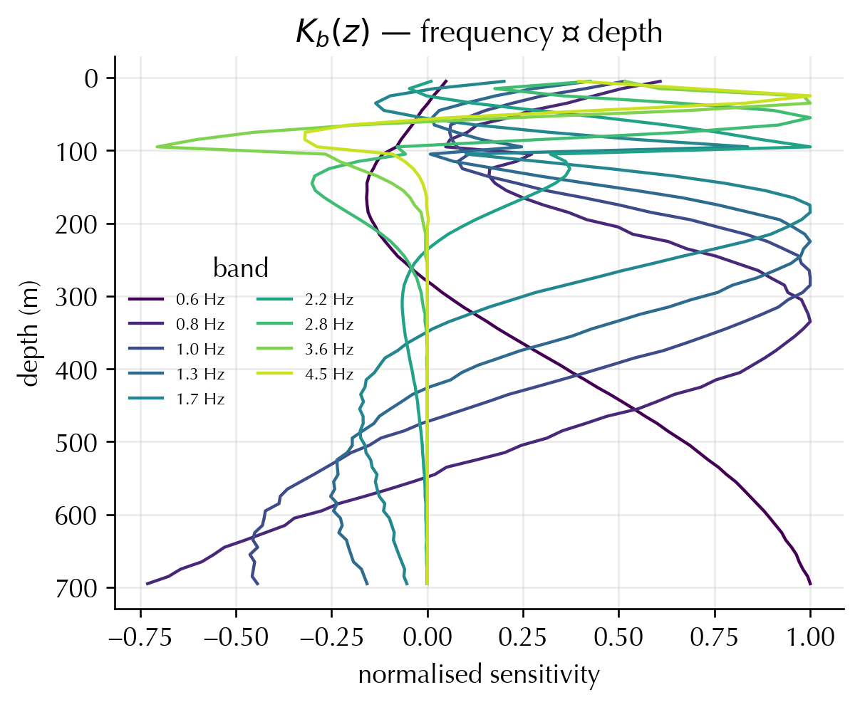
A band does not see a depth; it sees a **kernel** $K_b(z)$ — the Rayleigh-wave
sensitivity of that band, computed here with `disba` through
`band_sensitivity_matrix`. Low frequencies sense deep and broad; high
frequencies sense shallow and sharp. Stacking the kernels is the forward
operator $d = G\,m$ with $m(z)=\delta V_S/V_S(z)$.
```{python}
#| label: kernels
site = build_parkfield_site()
th, vp, vs, rho = site.velocity_model.to_arrays()
fine = make_fine_model(th, vp, vs, rho, target_dz_km=0.01, max_depth_km=1.5)
K = band_sensitivity_matrix(fine, bands, max_depth_km=0.7)
print("design G:", K.G.shape, "(bands × depths)")
print("peak sensitivity depth per band (m):",
      np.round(K.peak_depths_km * 1e3).astype(int))
```
```{python}
#| label: fig-kernels
#| fig-cap: "The band sensitivity kernels K_b(z) (area-normalised). Each band is a depth-weighting function; the set spans ~30–470 m here. This is the bridge that turns a *frequency*-domain error budget into a *depth*-domain one — and why you want several bands, not one."
fig, ax = plt.subplots(figsize=(5.5, 4.2))
zc = K.depths_km * 1e3
cmap = plt.cm.viridis(np.linspace(0, 0.92, len(bands)))
for b in range(len(bands)):
    ax.plot(K.G[b] / np.abs(K.G[b]).max(), zc, color=cmap[b], lw=1.3,
            label=f"{bands[b]:.1f} Hz")
ax.invert_yaxis()
ax.set(xlabel="normalised sensitivity", ylabel="depth (m)",
       title="$K_b(z)$ — frequency → depth")
ax.legend(fontsize=7, frameon=False, ncol=2, title="band")
plt.show()
```
## 4. Propagating the error into a depth profile
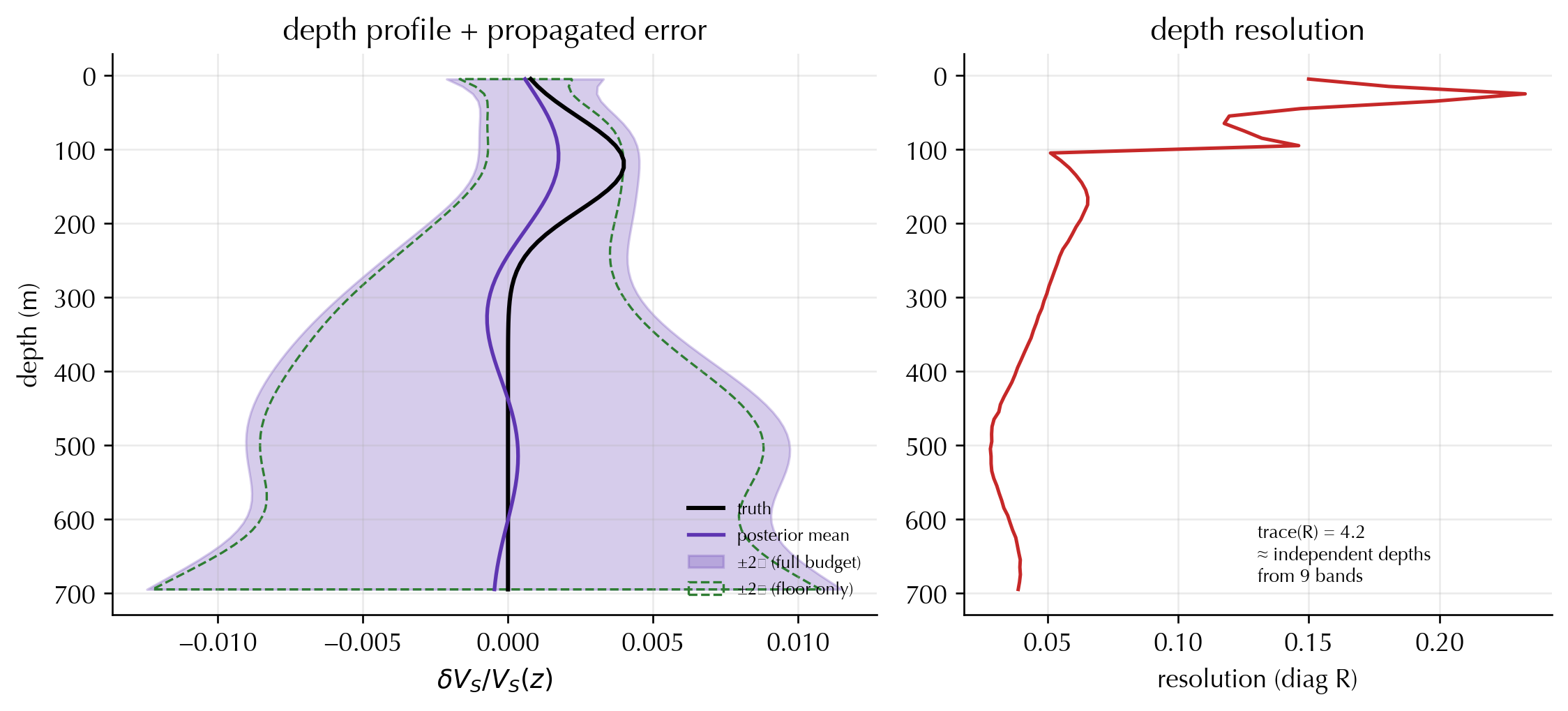
The final step feeds the per-band $\delta v/v$ and the per-band measurement
covariance $C_d$ (built from §2) into a Bayesian linear inversion,
$$
\hat C_m = (G^\top C_d^{-1} G + C_{m0}^{-1})^{-1},\qquad
\hat m = \hat C_m\, G^\top C_d^{-1}\, d,
$$ {#eq-depthinv}
(`invert_depth_profile`, with a smoothness prior $C_{m0}$). The **measurement
error — including the processing-choice part — flows straight into the depth
uncertainty** $\sqrt{\operatorname{diag}\hat C_m}$.
```{python}
#| label: invert
# a true velocity-change anomaly at ~120 m depth (e.g. a shallow pore-pressure pulse)
z = K.depths_km
m_true = 4e-3 * np.exp(-(((z - 0.12) / 0.09) ** 2))
d_clean = K.G @ m_true

sigma_band = np.array([pbe[float(f)]["total"] for f in bands])
# floor-only budget = ignore the processing-choice spread (the naive approach)
sigma_floor = np.array([pbe[float(f)]["within"] for f in bands])

# a fresh, fixed noise draw for a reproducible figure (one realisation)
noise_rng = np.random.default_rng(7)
d_obs = d_clean + sigma_band * noise_rng.standard_normal(len(bands))
post_full  = invert_depth_profile(d_obs, np.diag(sigma_band**2), K,
                                  prior_std=8e-3, corr_length_km=0.12)
post_floor = invert_depth_profile(d_obs, np.diag(sigma_floor**2), K,
                                  prior_std=8e-3, corr_length_km=0.12)
print(f"depth of recovered peak : {z[np.argmax(post_full.mean)]*1e3:.0f} m (truth 120 m)")
print(f"mean depth σ, full budget : {post_full.std.mean():.2e}")
print(f"mean depth σ, floor only  : {post_floor.std.mean():.2e}  "
      f"(under-reported by {post_full.std.mean()/post_floor.std.mean():.2f}×)")
```
```{python}
#| label: fig-depth
#| fig-cap: "The propagated depth result for one noise realisation. The posterior mean (purple) recovers the shallow anomaly; the dark band is the ±2σ uncertainty with the *full* processing-choice budget, the light dashed band is what you would report from the within-method floor alone. Ignoring the processing choices under-states the depth uncertainty — most in the shallow section probed by the high-frequency bands, where the windows are shortest and the estimators diverge most. The envelope is wide because a few bands resolve only a few depths; some realisations misplace the peak entirely, which is exactly why the ±2σ band — not the mean — is the result."
fig, ax = plt.subplots(1, 2, figsize=(9.5, 4.4), gridspec_kw={"width_ratios":[1.3,1]})
zc = z * 1e3
ax[0].plot(m_true, zc, color="k", lw=1.8, label="truth")
ax[0].plot(post_full.mean, zc, color=C["band"], lw=1.6, label="posterior mean")
ax[0].fill_betweenx(zc, post_full.mean-2*post_full.std, post_full.mean+2*post_full.std,
                    color=C["band"], alpha=0.25, label="±2σ (full budget)")
ax[0].fill_betweenx(zc, post_floor.mean-2*post_floor.std, post_floor.mean+2*post_floor.std,
                    facecolor="none", edgecolor=C["fit"], ls="--", lw=1.0,
                    label="±2σ (floor only)")
ax[0].invert_yaxis()
ax[0].set(xlabel=r"$\delta V_S/V_S(z)$", ylabel="depth (m)", title="depth profile + propagated error")
ax[0].legend(fontsize=7.5, frameon=False, loc="lower right")
# resolution: diagonal of R shows how well each depth is independently resolved
ax[1].plot(np.diag(post_full.resolution), zc, color=C["thermo"], lw=1.5)
ax[1].invert_yaxis()
ax[1].set(xlabel="resolution (diag R)", title="depth resolution")
ax[1].text(0.5, 0.05, f"trace(R) = {np.trace(post_full.resolution):.1f}\n"
           f"≈ independent depths\nfrom {len(bands)} bands",
           transform=ax[1].transAxes, fontsize=8, va="bottom")
plt.tight_layout(); plt.show()
```
::: {.callout-important}
Two lessons the resolution panel makes concrete. **First**, a handful of bands
resolves only a handful of independent depths ($\mathrm{trace}\,R\approx$ the
band count) — depth inversion from $\delta v/v$ is inherently low-resolution, and
honesty about that is part of the uncertainty. **Second**, the gap between the
two envelopes *is* the cost of pretending the processing choice was fixed.
:::
## 5. The full chain
```{mermaid}
flowchart LR
    RAW["repeated coda"]
    PRIOR["p(c): window rule,<br/>length, start, band"]
    SAMPLE["sample c ~ p(c)<br/>(multiverse)"]
    BAND["per-band σ_b<br/>floor ⊕ choice spread"]
    KERN["kernels K_b(z)<br/>(disba)"]
    CD["measurement<br/>covariance C_d"]
    INV["depth inversion<br/>m(z), Ĉ_m"]
    OUT["δV_S/V_S(z)<br/>+ honest envelope"]
    RAW --> SAMPLE
    PRIOR --> SAMPLE --> BAND --> CD
    BAND --> KERN
    KERN --> INV
    CD --> INV --> OUT
    style PRIOR fill:#fff3e0,stroke:#c77700
    style CD fill:#ede7f6,stroke:#5e35b1
    style OUT fill:#e8f5e9,stroke:#2e7d32
```
The processing choices enter as a **prior**, are **sampled** and marginalised
into one error per band, and — through the sensitivity kernels — propagate into
a depth profile whose uncertainty *finally* reflects what was actually unknown:
the measurement noise, **and** the freedom in how the measurement was made. This
is the depth-domain counterpart of the data covariance $C_d$ that the
[inference page](theory-uq.qmd) consumes.
## Partial saturation: $\delta V_S/V_S$ is not the only contribution
The inversion above assumes the change it recovers is a shear-velocity change
alone. In partially saturated ground it is not. Filling or draining pore space
changes both the shear modulus and the bulk density, so for the shear-dominated
coda the observed change mixes the two,
$$
\frac{\delta v}{v} \;\approx\; \tfrac12\frac{\delta\mu}{\mu} \;-\; \tfrac12\frac{\delta\rho}{\rho},
$$
and velocity alone cannot separate them. A petrophysical model — Gassmann fluid
substitution for the modulus and a porosity–saturation relation for the density
[@Gassmann1951; @Mavko2009] — is what breaks the degeneracy, at the cost
of its own prior uncertainty on porosity, fluid modulus, and the saturation path.
Hydrological and cryospheric targets, where saturation swings are large
[@Clements2018; @James2019], are precisely where neglecting the
density term biases the inferred velocity change and, downstream, the stress.
The planned extension carries $\delta\rho/\rho$ as a **second inverted field**
with its own kernel and reports how much of the surface $\delta v/v$ each field
explains, propagating the saturation and porosity prior into the split. This is
tracked as open development — a `codameter` Gassmann / partial-saturation module
and its synthetic demo (see the repository issues) — and it is the depth-step
input the [stress page](uncertainty-3-stress.qmd) needs before effective stress
can be trusted in unsaturated ground.
---
::: {.callout-tip}
## Where this lives in the code
- @eq-flatten → `codameter.uq_processing.flatten_end_lapse`
- §2 sampling / @eq-ltv → `ProcessingPrior`, `sample_processing_choices`, `per_band_marginal_error`
- §3 kernels → `codameter.uq_depth.band_sensitivity_matrix` (built on `codameter.kernels`, `disba`)
- @eq-depthinv → `codameter.uq_depth.invert_depth_profile` → `DepthProfilePosterior`
:::
### References {.unnumbered}
::: {#refs}
:::