---
title: "0 · Measuring δv/v from noisy cross-correlations"
subtitle: "A realistic CCF gather → δv/v(t), its uncertainty over time, and the covariance C_d"
jupyter: codameter-pixi
bibliography: references.bib
format:
html: default
ipynb: default
---
[⬇ Download this tutorial as a Jupyter notebook](tutorial-00-measurement.ipynb){.btn .btn-outline-primary .btn-sm role="button" download=""}
::: {.keyidea}
[Thesis]{.k-title}
Every other tutorial starts from a $\delta v/v$ *series*. This one starts one step
earlier — from the **raw daily cross-correlations**, the actual input. We build a
CCF gather that carries the nuisances real data does (a slow velocity change, finite
SNR, an instrument **clock drift**, and a **seasonal** noise-source wobble in the
late coda), then use `codameter` to recover $\delta v/v(t)$, **its uncertainty over
time**, and the **measurement covariance** $C_d$ — the exact object
[step 2 · depth](theory-processing-depth.qmd) consumes. It is the hands-on companion
to the [marginal-errors](theory-measurement-uq.qmd) and
[Bayesian-measurement](theory-bayesian-measurement.qmd) theory pages.
:::
```{python}
#| label: setup
import sys, numpy as np, matplotlib.pyplot as plt
sys.path.insert(0, ".")
from _synth import set_style, C
set_style()
from codameter.synthetic_demo import (
    Synth, _days, volcano_truth, daily_ccfs,
    add_clock_drift, add_seasonal_late_noise,
    stretching_cc, peak_dvv, measure_stretching, YEAR_D,
)
from codameter.uq_measurement import weaver_stretching_error
from codameter import uq_bayes as B
rng = np.random.default_rng(3)
```
## 1. A realistic cross-correlation gather
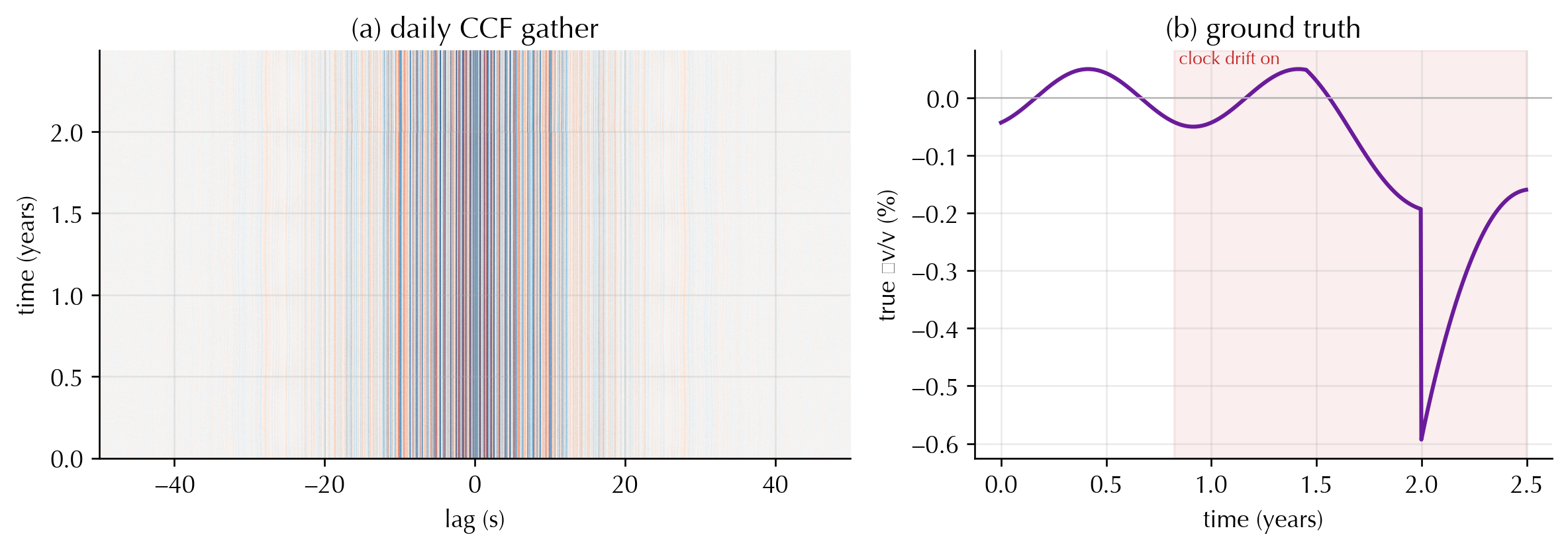
We assemble the data the way a monitoring station delivers it: one reference coda
and a stack of **daily** cross-correlations, each a noisy repeat of that reference
with a small, slowly changing stretch. On top of the true velocity change we layer
three nuisances that a real record almost always contains:
- **A long-term velocity change** — a slow pre-eruptive decline, a sharp
co-eruptive drop, then recovery (`volcano_truth`). This is the signal, and it is
the *long-term shifting of the coda phases* we want to recover.
- **Measurement noise** — a finite coda-to-noise ratio (`snr`), the irreducible
per-day scatter.
- **An instrument clock drift** — a station-timing error that delays the *whole*
correlation by a lag that grows with time (`add_clock_drift`). It mimics a real
velocity change but, being a constant lag, betrays itself on the two coda
branches (§2).
- **A seasonal noise-source wobble** — a seasonally changing noise field that warps
only the **late** coda (`add_seasonal_late_noise`), injecting a spurious seasonal
$\delta v/v$ into a late measurement window but not an early one.
```{python}
#| label: build
s = Synth()                       # shared coda geometry: lag axis s.t, reference s.ref
days = _days(2.5)                 # ~2.5 years of daily CCFs
truth = volcano_truth(days)       # the ground-truth δv/v(t)

# start from clean daily CCFs at a realistic SNR ...
ccfs = daily_ccfs(s.t, [s.ref], [truth], fs=s.fs, snr=7.0, seed=55)
# ... then contaminate them the way nature does:
ccfs = add_clock_drift(ccfs, s.t, drift_s_per_day=5e-5, onset_day=300)
ccfs = add_seasonal_late_noise(ccfs, s.t, days, fs=s.fs, onset_s=25.0,
                               dvv_amp=0.0035, jitter=0.05, seed=9)
print(f"gather: {ccfs.shape[0]} daily CCFs × {ccfs.shape[1]} lag samples "
      f"(±{s.maxlag_s:g} s at {s.fs:g} Hz)")
```
```{python}
#| label: fig-gather
#| fig-cap: "The synthetic gather. (a) The stack of daily cross-correlations (lag × time); the coda structure repeats day to day, and the imposed changes are a fraction of a percent — invisible by eye, which is the whole problem. (b) The ground truth we are trying to recover: a slow decline, a co-eruptive drop at year 2, and recovery. The clock drift (from day 300) and the seasonal wobble are the nuisances layered on top."
fig, ax = plt.subplots(1, 2, figsize=(10, 3.6), gridspec_kw={"width_ratios": [1.3, 1]})
yrs = days / YEAR_D
vmax = np.percentile(np.abs(ccfs), 99)
ax[0].imshow(ccfs, aspect="auto", origin="lower", cmap="RdBu_r", vmin=-vmax, vmax=vmax,
             extent=[s.t[0], s.t[-1], yrs[0], yrs[-1]])
ax[0].set(xlabel="lag (s)", ylabel="time (years)", title="(a) daily CCF gather")
ax[1].plot(yrs, truth * 100, color=C["damage"], lw=1.8)
ax[1].axvspan(300 / YEAR_D, yrs[-1], color=C["thermo"], alpha=0.08)
ax[1].text(300 / YEAR_D, ax[1].get_ylim()[1], " clock drift on", color=C["thermo"],
           fontsize=8, va="top")
ax[1].axhline(0, color="0.7", lw=0.7)
ax[1].set(xlabel="time (years)", ylabel="true δv/v (%)", title="(b) ground truth")
plt.tight_layout(); plt.show()
```
## 2. Measure δv/v — and watch the nuisances bite
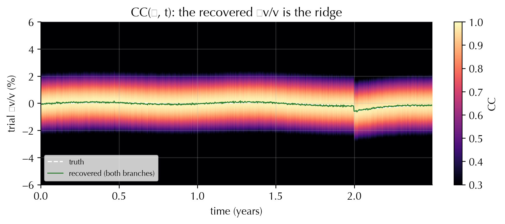
The workhorse is **trace stretching**: for each day, find the stretch $\varepsilon$
of the reference coda that best matches the current trace over a lapse window. The
`stretching_cc` helper returns the full correlation image $\mathrm{CC}(\varepsilon,t)$;
its bright ridge *is* the apparent $\delta v/v(t)$.
```{python}
#| label: fig-ccimage
#| fig-cap: "The stretching correlation image CC(ε, t) over a late coda window [8, 35] s. The bright ridge is the recovered δv/v(t). It shows the true decline and drop — but also a slow upward creep after day 300 (the clock drift) and a faint annual wobble (the seasonal late-coda noise). Raw, a single late-window stretch conflates all three."
band, window = (0.4, 1.0), (8.0, 35.0)
es, cc_img = stretching_cc(ccfs, s.ref, s.t, band=band, fs=s.fs, window=window)
dvv_both, cc_peak = peak_dvv(es, cc_img)

fig, ax = plt.subplots(figsize=(7.5, 3.4))
im = ax.imshow(cc_img.T, aspect="auto", origin="lower", cmap="magma",
               extent=[yrs[0], yrs[-1], es[0] * 100, es[-1] * 100], vmin=0.3, vmax=1.0)
ax.plot(yrs, truth * 100, color="w", lw=1.2, ls="--", label="truth")
ax.plot(yrs, dvv_both * 100, color=C["fit"], lw=1.0, label="recovered (both branches)")
ax.set(xlabel="time (years)", ylabel="trial δv/v (%)",
       title="CC(ε, t): the recovered δv/v is the ridge")
ax.legend(fontsize=8, loc="lower left"); fig.colorbar(im, ax=ax, fraction=0.046, label="CC")
plt.tight_layout(); plt.show()
```
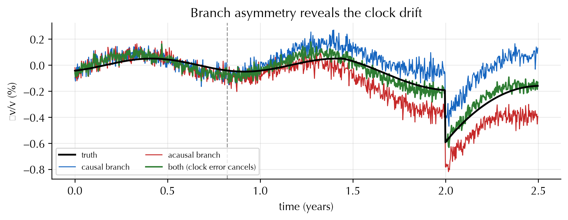
**The clock-drift diagnostic.** A clock error delays the whole correlation by a
constant lag, so it looks like a *slowing* on the causal (positive-lag) branch and a
*speeding* on the acausal branch — opposite signs. A true velocity change moves both
the same way. Measuring the two branches separately exposes it; using **both**
branches together averages it away.
```{python}
#| label: fig-branches
#| fig-cap: "Measuring each coda branch separately is the clock-error diagnostic. After day 300 the causal and acausal δv/v split symmetrically (the clock drift, opposite sign on each), while their average — the 'both-branch' measurement — cancels it and tracks the truth. A single-branch pipeline would mistake the clock drift for a real velocity change."
dvv_c, _ = measure_stretching(ccfs, s.ref, s.t, band=band, fs=s.fs, window=window, branch="causal")
dvv_a, _ = measure_stretching(ccfs, s.ref, s.t, band=band, fs=s.fs, window=window, branch="acausal")

fig, ax = plt.subplots(figsize=(8, 3.2))
ax.plot(yrs, truth * 100, color="k", lw=1.8, label="truth", zorder=5)
ax.plot(yrs, dvv_c * 100, color=C["hydro"], lw=0.9, label="causal branch")
ax.plot(yrs, dvv_a * 100, color=C["thermo"], lw=0.9, label="acausal branch")
ax.plot(yrs, dvv_both * 100, color=C["fit"], lw=1.4, label="both (clock error cancels)")
ax.axvline(300 / YEAR_D, color="0.6", ls="--", lw=1)
ax.set(xlabel="time (years)", ylabel="δv/v (%)", title="Branch asymmetry reveals the clock drift")
ax.legend(fontsize=8, ncol=2); plt.tight_layout(); plt.show()
```
## 3. The uncertainty over time
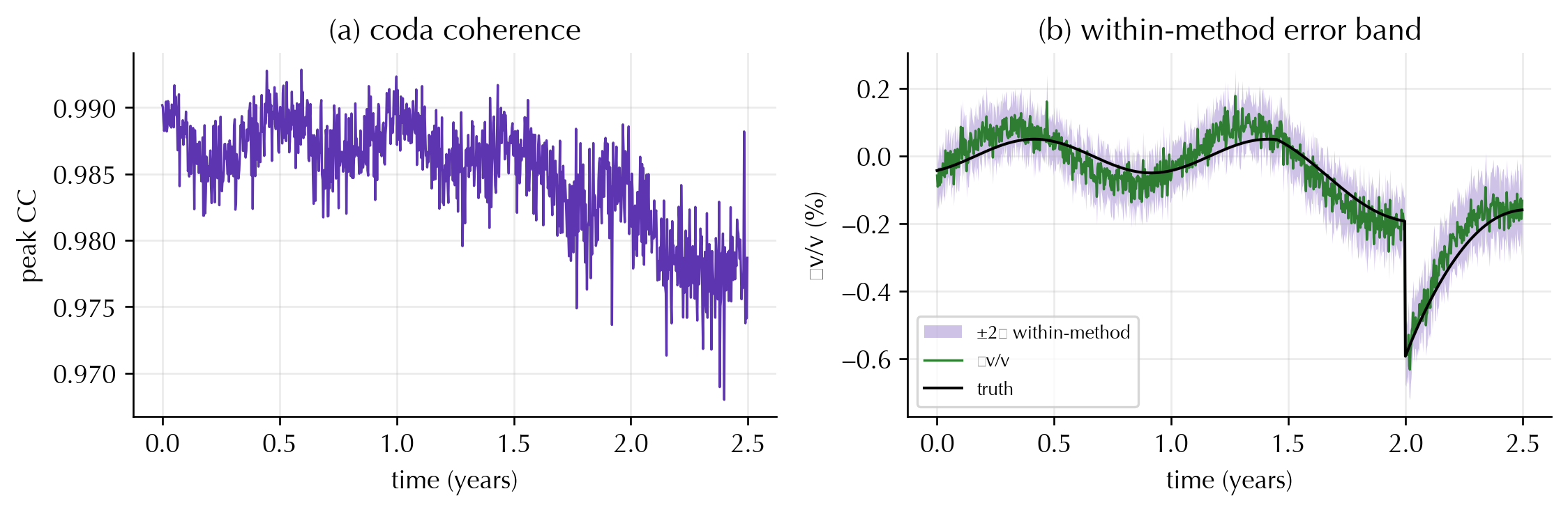
A single number per epoch is not enough — the error is **time-dependent**. The
irreducible *within-method floor* comes from the coda coherence: where the current
trace correlates poorly with the reference (the low-SNR days, and especially the
sharp co-eruptive drop), the stretching estimate is less certain. The
`weaver_stretching_error` formula turns the peak correlation $\mathrm{CC}(t)$ into a
per-epoch standard error.
```{python}
#| label: fig-floor
#| fig-cap: "The coherence-limited error floor. Where the peak CC dips — the noisy stretch around the co-eruptive drop at year 2 — the within-method σ spikes. This is the floor a single pipeline would report; §4 shows it is only part of the story."
fc = float(np.sqrt(band[0] * band[1]))              # band centre
sig_within = weaver_stretching_error(cc_peak, fc, window[0], window[1])

fig, ax = plt.subplots(1, 2, figsize=(9.5, 3.2), gridspec_kw={"width_ratios": [1, 1]})
ax[0].plot(yrs, cc_peak, color=C["accent"], lw=1.0)
ax[0].set(xlabel="time (years)", ylabel="peak CC", title="(a) coda coherence")
ax[1].fill_between(yrs, (dvv_both - 2 * sig_within) * 100, (dvv_both + 2 * sig_within) * 100,
                   color=C["band"], alpha=0.3, lw=0, label="±2σ within-method")
ax[1].plot(yrs, dvv_both * 100, color=C["fit"], lw=1.0, label="δv/v")
ax[1].plot(yrs, truth * 100, color="k", lw=1.2, label="truth")
ax[1].set(xlabel="time (years)", ylabel="δv/v (%)", title="(b) within-method error band")
ax[1].legend(fontsize=8); plt.tight_layout(); plt.show()
```
## 4. The measurement covariance $C_d$
The within-method floor assumes *one* pipeline is correct. It is not: the estimator,
band, and window are all defensible-but-different choices, and their spread is a
genuine, usually dominant, uncertainty. `codameter` marginalises that choice — it
runs an ensemble of pipelines on the same gather and folds their spread, the
coherence floor, and the temporal correlation into one **time-dependent measurement
covariance** $C_d$. One call does the whole thing:
```{python}
#| label: bayes
res, run = B.bayes_dvv_from_ccfs(ccfs, s.t, s.fs, truth=truth, days=days,
                                 cadence=4, n_iter=1200, burn=400, thin=2)
print(f"ensemble                     : {run.members.shape[0]} pipelines")
print(f"methodological bias scale τ  : {res.tau:.2e}")
print(f"Weaver-floor rescale s       : {res.s:.2f}   (>1 ⇒ the raw floor is optimistic)")
print(f"temporal correlation length  : {res.corr_length_days:.0f} days")
print(f"effective sample size  N_eff : {res.n_eff:.0f} of {len(res.times_days)} epochs")
```
```{python}
#| label: fig-cd
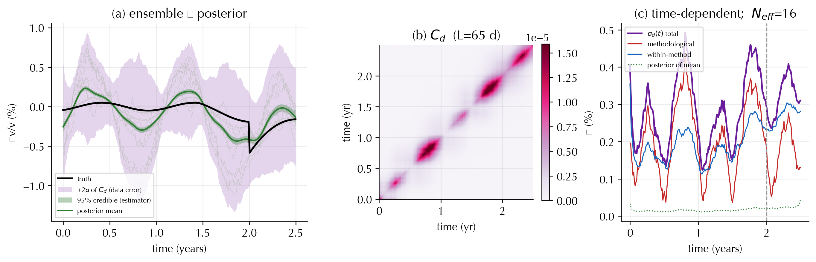
#| fig-cap: "The deliverable. (a) The pipeline ensemble (grey) marginalised into a posterior mean (purple); its 95% credible band is the *estimator* precision — narrow, and it under-covers the truth — while the ±2σ band of C_d is the honest measurement error. (b) The measurement covariance C_d itself: a time-dependent diagonal with an exponential temporal correlation and a common-mode floor. (c) σ_d(t) split into within-method and methodological parts — both widen at the eruption — with N_eff collapsed far below the epoch count."
yrs_e = res.times_days / YEAR_D
sd_cd = np.sqrt(np.diag(res.Cd)); sd_post = np.sqrt(np.diag(res.mu_cov))
fig = plt.figure(figsize=(11.5, 3.8))
gs = fig.add_gridspec(1, 3, width_ratios=[1.5, 1.0, 1.1])

ax0 = fig.add_subplot(gs[0])
for k in range(run.members.shape[0]):
    ax0.plot(yrs_e, run.members[k] * 100, lw=0.5, color="0.75", alpha=0.6)
ax0.plot(yrs_e, run.truth * 100, color="k", lw=1.8, label="truth", zorder=6)
ax0.fill_between(yrs_e, (res.mu_mean - 2 * sd_cd) * 100, (res.mu_mean + 2 * sd_cd) * 100,
                 color=C["damage"], alpha=0.18, lw=0, label=r"±2σ of $C_d$ (data error)")
ax0.fill_between(yrs_e, res.mu_lo * 100, res.mu_hi * 100, color=C["fit"], alpha=0.35, lw=0,
                 label="95% credible (estimator)")
ax0.plot(yrs_e, res.mu_mean * 100, color=C["fit"], lw=1.5, label="posterior mean")
ax0.set(xlabel="time (years)", ylabel="δv/v (%)", title="(a) ensemble → posterior")
ax0.legend(fontsize=7, loc="lower left")

ax1 = fig.add_subplot(gs[1])
vmax = float(np.percentile(np.diag(res.Cd), 85))
im = ax1.imshow(res.Cd, cmap="PuRd", origin="lower", vmin=0, vmax=vmax,
                extent=[yrs_e[0], yrs_e[-1], yrs_e[0], yrs_e[-1]])
ax1.set(title=f"(b) $C_d$  (L={res.corr_length_days:.0f} d)",
        xlabel="time (yr)", ylabel="time (yr)")
fig.colorbar(im, ax=ax1, fraction=0.046)

ax2 = fig.add_subplot(gs[2])
ax2.plot(yrs_e, sd_cd * 100, color=C["damage"], lw=1.6, label=r"$\sigma_d(t)$ total")
ax2.plot(yrs_e, res.method_std * 100, color=C["thermo"], lw=1.0, label="methodological")
ax2.plot(yrs_e, res.within_std * 100, color=C["hydro"], lw=1.0, label="within-method")
ax2.plot(yrs_e, sd_post * 100, color=C["fit"], lw=1.0, ls=":", label="posterior of mean")
ax2.axvline(2.0, color="0.6", ls="--", lw=1)
ax2.set(xlabel="time (years)", ylabel="σ (%)",
        title=f"(c) time-dependent;  $N_{{eff}}$={res.n_eff:.0f}")
ax2.legend(fontsize=7); plt.tight_layout(); plt.show()
```
```{python}
#| label: coverage
tr = run.truth
cred = np.mean((tr >= res.mu_lo) & (tr <= res.mu_hi))
cd95 = np.mean(np.abs(tr - res.mu_mean) <= 2 * sd_cd)
print(f"truth inside 95% credible band : {cred:.0%}   (the estimator precision under-covers)")
print(f"truth within ±2σ of C_d        : {cd95:.0%}   (the honest measurement error covers)")
print(f"mean σ: credible {sd_post.mean():.2e}  vs  C_d {sd_cd.mean():.2e}  "
      f"({sd_cd.mean() / sd_post.mean():.0f}× wider)")
```
The credible band — the precision of the *combined* estimate — is tight and
over-confident; the marginal covariance $C_d$ is what actually covers the truth. That
gap is the point: report and **propagate $C_d$**, not the posterior of the averaged
series.
## What you produced, and where it goes
From a raw, contaminated CCF gather you now have the three objects the rest of the
arc needs:
1. a marginalised $\delta v/v(t)$ (`res.mu_mean`),
2. its time-dependent standard error $\sigma_d(t)$ (`np.sqrt(np.diag(res.Cd))`), and
3. the full measurement covariance $C_d$ (`res.Cd`), with its temporal correlation
and common-mode floor.
$C_d$ is exactly the input [step 2 · depth](theory-processing-depth.qmd) inverts
through sensitivity kernels for a profile of shear-velocity change — and an honest
depth or stress estimate is only as honest as the $C_d$ it starts from. The clock
error we diagnosed here is a reminder that some systematics (timing, a
non-stationary noise field) must be **detected and removed before** measuring;
what remains — coherence, and the freedom in the processing choice — is what $C_d$
carries forward.
### References {.unnumbered}
::: {#refs}
:::