The marginal errors in δv/v, and how they differ

The within-method floor, the methodological spread, temporal correlation, and reference choice — and where each dominates

Thesis This is step 1 of the uncertainty arc. A \(\delta v/v\) series is the end of a long chain of processing choices (method, window, band, stacking, gating, reference), almost none of which are propagated — and it is the least reproducible step in the discipline. This page maps the marginal errors in that series and shows how they differ: the within-method coherence floor, the methodological spread across processing choices, their temporal correlation, and the shift from the reference choice — and where each one dominates. Its deliverable is not a scalar per epoch but a structured measurement covariance \(C_d\), the object step 2 · depth and step 3 · stress consume. The companion page then turns these marginal errors into a single Bayesian measurement.

Where the field stands

The community agrees on the components of a well-posed measurement — a stretching-family estimator for robustness at low SNR and large change (Mikesell et al. 2015; Yuan et al. 2021), a coherence-based error model (Clarke et al. 2011; Weaver et al. 2011), a long stable reference (Wang et al. 2017), and cross-validation against a second estimator (Obermann and Hillers 2019) — yet no two studies report the same set, and the uncertainty convention is the least standardized of all (literature survey). Propagating the measurement covariance matters because everything downstream in the arc consumes it: a depth profile or a stress estimate is only as honest as the \(C_d\) it starts from. The table pairs each choice with its documented deviation and the consequence; it is the source the executable codameter.deviations menu draws from.

Choice Best practice Common deviation Consequence
Estimator Stretching family, robust at low SNR / large δv/v Bare MWCS / wrapped phase Cycle-skips at large δv/v; error ~10× or catastrophic
Frequency band Band matched to the target depth Off-target or single wide band Mixes depths; mostly sets precision
Coda window Past the direct arrival, scaled with the band Fixed late window reused across bands Noise at high f; bias, inflated σ
Stack length Short enough to resolve the transient (~10 d) Over-long stack (~45 d) Smears and delays a step
Reference Long fixed stack or joint inversion (Brenguier et al. 2014) Moving / trailing reference Erases slow trends
Coherence gating Discard low-coherence epochs No gating Keeps corrupted epochs; changes Neff
Uncertainty definition State it: within-measurement / SE / SD Left unstated Factor √N ambiguity in significance
Code
import sys, numpy as np, matplotlib.pyplot as plt
sys.path.insert(0, ".")
from _synth import set_style, C
set_style()
from codameter.uq_measurement import (
    weaver_stretching_error, processing_ensemble, temporal_error_covariance,
    effective_sample_size, global_reference_inversion, single_reference_dvv)
rng = np.random.default_rng(7)

1. The \(\delta v/v\) measurement is a tree of choices

A \(\delta v/v\) value is not measured; it is computed from a stack of repeated coda waves through a pipeline. Each fork is a reasonable choice, and different groups fork differently — so the same raw data yields different \(\delta v/v(t)\).

Code
flowchart LR
    RAW["repeated coda<br/>(cross-correlations)"]
    STACK{"stack?<br/>linear / PWS<br/>substack length"}
    GATE{"gate?<br/>discard CC &lt; thresh"}
    REF{"reference?<br/>fixed / trailing /<br/>all-to-all"}
    METH{"estimator?<br/>stretching / MWCS /<br/>wavelet / DTW"}
    WIN{"window?<br/>coda start, length,<br/>frequency band"}
    DVV["δv/v(t)<br/>+ what error?"]
    RAW --> STACK --> GATE --> REF --> METH --> WIN --> DVV
    style DVV fill:#fce4ec,stroke:#c62828
    style REF fill:#fff3e0,stroke:#c77700

flowchart LR
    RAW["repeated coda<br/>(cross-correlations)"]
    STACK{"stack?<br/>linear / PWS<br/>substack length"}
    GATE{"gate?<br/>discard CC &lt; thresh"}
    REF{"reference?<br/>fixed / trailing /<br/>all-to-all"}
    METH{"estimator?<br/>stretching / MWCS /<br/>wavelet / DTW"}
    WIN{"window?<br/>coda start, length,<br/>frequency band"}
    DVV["δv/v(t)<br/>+ what error?"]
    RAW --> STACK --> GATE --> REF --> METH --> WIN --> DVV
    style DVV fill:#fce4ec,stroke:#c62828
    style REF fill:#fff3e0,stroke:#c77700

We treat each fork as a source of measurement uncertainty and quantify three things a diagonal dvv_err cannot express: a within-method floor, a methodological spread, and the temporal correlation the choices induce.

2. The coherence-limited within-method floor

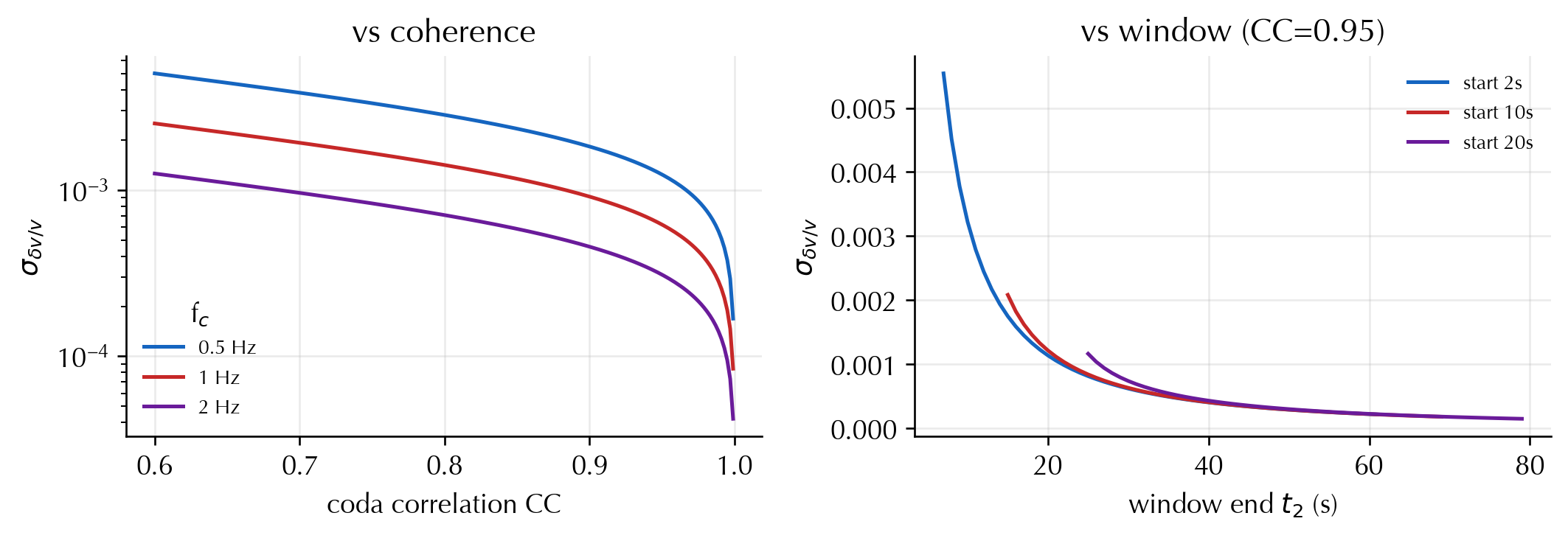
For a fixed configuration there is an irreducible scatter set by the coda coherence. Weaver et al. (2011) and Clarke et al. (2011) give the standard error of a stretching/MWCS estimate over a coda window \([t_1,t_2]\) with mean correlation \(CC\) at central frequency \(f_c\):

\[ \sigma_{\delta v/v}^2 = \frac{1-CC^2}{2\,CC^2}\; \frac{6\sqrt{\pi/2}}{\omega_c^2\,(t_2^3 - t_1^3)}, \qquad \omega_c = 2\pi f_c . \tag{1}\]

This is weaver_stretching_error. It encodes the levers practitioners actually turn: higher coherence, a longer/later coda window, and higher frequency all shrink the error — and it is the floor, achieved only if every other choice were fixed and correct.

Code
cc = np.linspace(0.6, 0.999, 200)
fig, ax = plt.subplots(1, 2, figsize=(9, 3.2))
for fc, col in [(0.5, C["hydro"]), (1.0, C["thermo"]), (2.0, C["damage"])]:
    ax[0].plot(cc, weaver_stretching_error(cc, fc, 5, 30), color=col, label=f"{fc:g} Hz")
ax[0].set(xlabel="coda correlation CC", ylabel=r"$\sigma_{\delta v/v}$",
          yscale="log", title="vs coherence")
ax[0].legend(fontsize=8, frameon=False, title="f$_c$")
lengths = np.arange(5, 60, 1.0)
for t1, col in [(2, C["hydro"]), (10, C["thermo"]), (20, C["damage"])]:
    s = [weaver_stretching_error(0.95, 1.0, t1, t1+L) for L in lengths]
    ax[1].plot(t1+lengths, s, color=col, label=f"start {t1}s")
ax[1].set(xlabel="window end $t_2$ (s)", ylabel=r"$\sigma_{\delta v/v}$",
          title="vs window (CC=0.95)")
ax[1].legend(fontsize=8, frameon=False)
plt.tight_layout(); plt.show()
Figure 1: The coherence-limited δv/v error floor (Weaver/Clarke). Left: error explodes as coda coherence drops — the basis for CC-gating. Right: a longer/later coda window lowers the floor (∝ 1/√(t₂³−t₁³)), the reason late-coda windows are prized despite lower SNR.

3. The methodological spread over choices

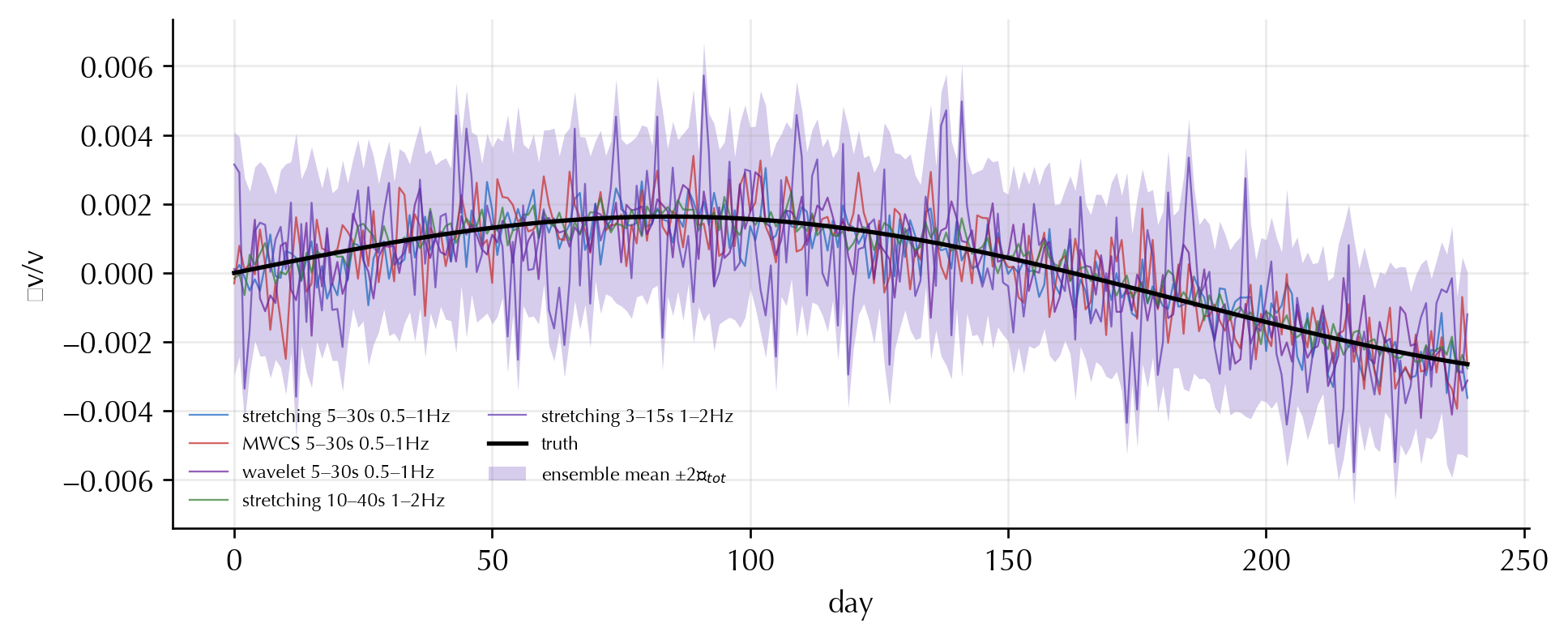
The floor assumes the configuration is the configuration. It is not. Run the same data through several reasonable pipelines and you get an ensemble of \(\delta v/v(t)\) curves whose spread is a genuine, usually dominant, uncertainty. We simulate that here: a common truth seen through stretching, MWCS, a wavelet estimator, and two window/band variants — each with its own bias and coherence-limited noise.

Code
n = 240
t_days = np.arange(n, dtype=float)
truth = 2e-3 * np.sin(2*np.pi*t_days/365.0) - 1e-3*(t_days/n)   # seasonal + trend

# each configuration: (multiplicative bias, additive bias, CC, window, fc)
configs = {
    "stretching 5–30s 0.5–1Hz": (1.00,  0.0e-4, 0.97, (5, 30), 0.7),
    "MWCS 5–30s 0.5–1Hz":       (0.93,  1.0e-4, 0.95, (5, 30), 0.7),
    "wavelet 5–30s 0.5–1Hz":    (1.05, -0.8e-4, 0.96, (5, 30), 0.7),
    "stretching 10–40s 1–2Hz":  (1.02,  0.4e-4, 0.93, (10, 40), 1.5),
    "stretching 3–15s 1–2Hz":   (0.97, -0.5e-4, 0.90, (3, 15), 1.5),
}
members, within = {}, {}
for name, (mb, ab, cc_, (t1, t2), fc) in configs.items():
    sig = float(weaver_stretching_error(cc_, fc, t1, t2))
    members[name] = mb*truth + ab + sig*rng.standard_normal(n)
    within[name] = np.full(n, sig)

ens = processing_ensemble(members, within)
print(f"mean within-method floor : {ens.within_std.mean():.2e}")
print(f"methodological spread     : {ens.methodological_std.mean():.2e}  "
      f"({ens.methodological_std.mean()/ens.within_std.mean():.1f}× the floor)")
print(f"total measurement error   : {ens.total_std.mean():.2e}")
mean within-method floor : 9.92e-04
methodological spread     : 8.81e-04  (0.9× the floor)
total measurement error   : 1.36e-03
Code
fig, ax = plt.subplots(figsize=(9, 3.4))
for name in ens.member_labels:
    ax.plot(t_days, members[name], lw=0.7, alpha=0.7, label=name)
ax.plot(t_days, truth, color="k", lw=1.6, label="truth", zorder=5)
ax.fill_between(t_days, ens.mean-2*ens.total_std, ens.mean+2*ens.total_std,
                color=C["band"], alpha=0.25, lw=0, label="ensemble mean ±2σ$_{tot}$")
ax.set(xlabel="day", ylabel="δv/v")
ax.legend(fontsize=7, frameon=False, ncol=2, loc="lower left")
plt.show()
Figure 2: The processing ensemble. Thin lines are individual pipelines; the band is the configuration-marginal mean ± the total measurement error (within-method floor combined with methodological spread by the law of total variance). The spread between methods dwarfs each method’s own error bar — the reproducibility problem in one figure.

4. Temporal correlation and the common-mode reference

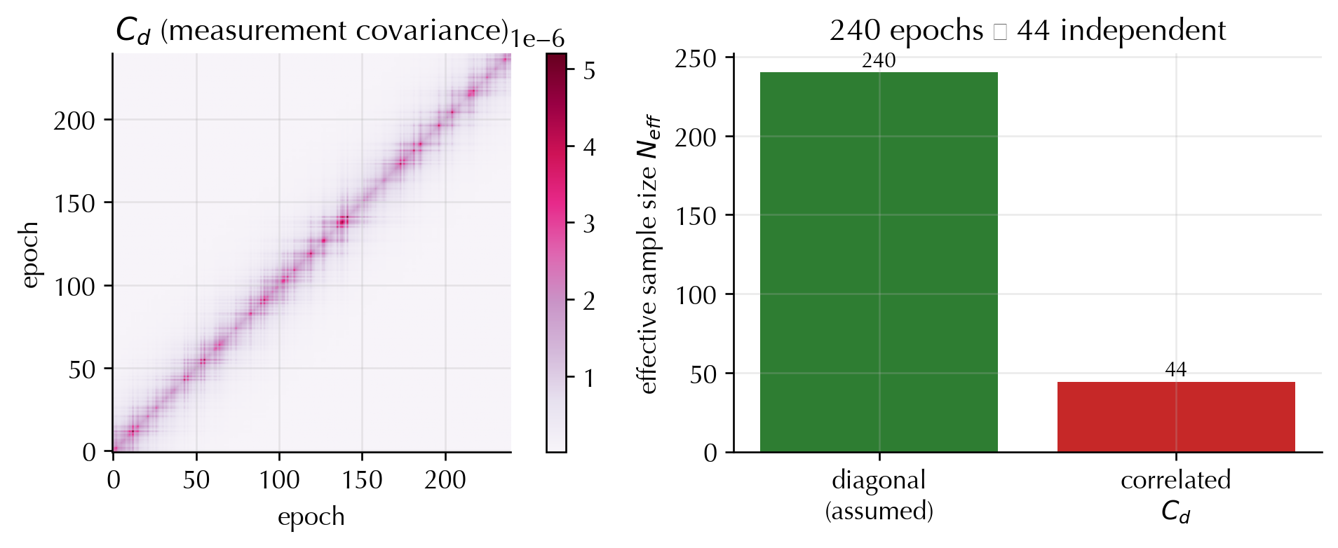
The errors above are not independent in time. Overlapping stacks share waveform data, so neighbouring epochs are correlated; and any single shared reference injects an error that is identical for every epoch — a fully correlated common-mode term. The honest measurement covariance is

\[ C_d = D\,R\,D \;+\; \sigma_{\rm ref}^2\,\mathbf{1}\mathbf{1}^\top, \qquad D=\operatorname{diag}(\sigma_{\rm tot}),\;\; R_{ij}=e^{-|t_i-t_j|/L}, \tag{2}\]

built by temporal_error_covariance. The off-diagonal structure matters enormously: it collapses the effective number of independent measurements.

Code
Cd = temporal_error_covariance(ens.total_std, t_days, corr_length_days=14.0,
                               common_mode_sigma=1.5e-4)
Cd_diag = np.diag(np.diag(Cd))
fig, ax = plt.subplots(1, 2, figsize=(9, 3.4),
                       gridspec_kw={"width_ratios": [1.2, 1]})
im = ax[0].imshow(Cd, cmap="PuRd", origin="lower")
ax[0].set(title="$C_d$ (measurement covariance)", xlabel="epoch", ylabel="epoch")
fig.colorbar(im, ax=ax[0], fraction=0.046)
neff_corr = effective_sample_size(Cd)
neff_diag = effective_sample_size(Cd_diag)
ax[1].bar(["diagonal\n(assumed)", "correlated\n$C_d$"], [neff_diag, neff_corr],
          color=[C["fit"], C["thermo"]])
ax[1].set(ylabel="effective sample size $N_{eff}$",
          title=f"{n} epochs → {neff_corr:.0f} independent")
for i, v in enumerate([neff_diag, neff_corr]):
    ax[1].text(i, v, f"{v:.0f}", ha="center", va="bottom", fontsize=9)
plt.tight_layout(); plt.show()
Figure 3: Left: the structured measurement covariance C_d — a banded temporal correlation (overlapping stacks, length L=14 d) plus a uniform common-mode floor from the shared reference. Right: the effective sample size for estimating a common level. The diagonal assumption returns the full count; the real correlation collapses it by more than an order of magnitude — and the collapse is dominated by the common-mode reference term, which (unlike random noise) does not average down. Reference choice, not sample count, sets the information.

5. Reference choice and the Brenguier et al. (2014) all-to-all cure

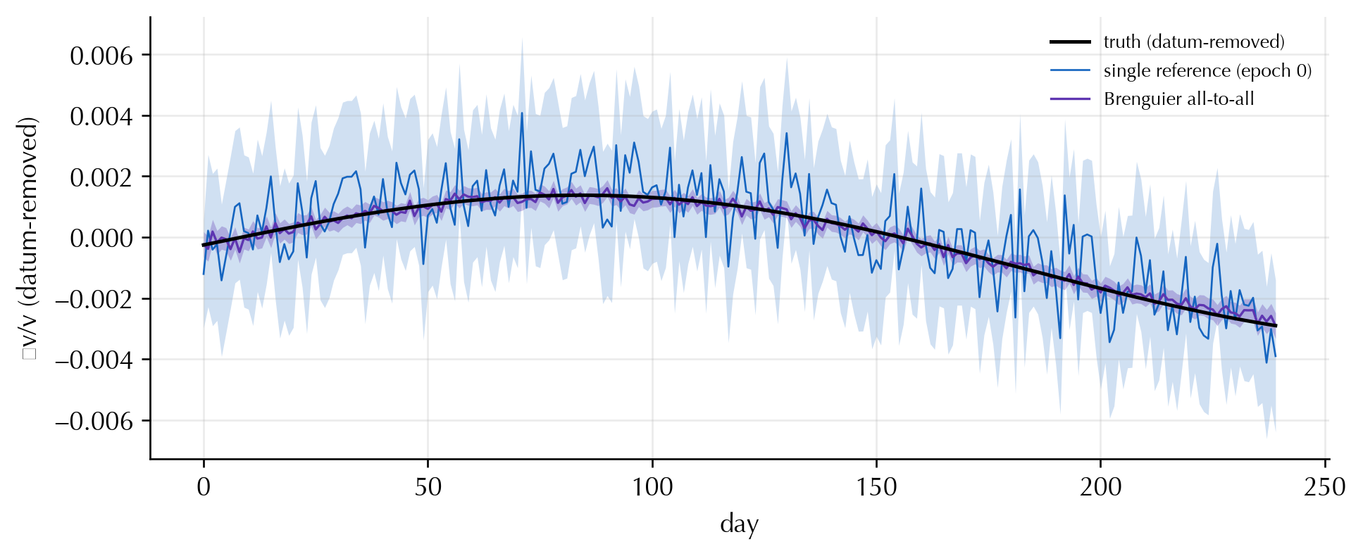
The most consequential — and least examined — fork is the reference. Referencing every epoch to one stack makes the reference’s own noise a common-mode error and ties the whole series to an arbitrary datum. Brenguier et al. (2014) showed a way out: treat every window as a reference, measure the relative velocity change between all pairs of epochs, and invert the double-difference system

\[ \varepsilon_{ij} = m_i - m_j + \eta_{ij}, \qquad \eta_{ij}\sim\mathcal N(0,\sigma_{ij}^2), \tag{3}\]

for a global, reference-free \(m=\delta v/v(t)\) (global_reference_inversion). Its model covariance \((G^\top C_d^{-1} G)^{+}\) is temporally correlated by construction — the principled \(C_d\) the reference choice implies.

Code
m_true = truth - truth.mean()          # the inversion resolves dv/v up to a datum
# (a) single fixed reference at epoch 0: every epoch measured against one stack
sig_ref = float(weaver_stretching_error(0.95, 0.7, 5, 30))
rel0 = (m_true - m_true[0]) + sig_ref*rng.standard_normal(n)
dvv_single, cov_single = single_reference_dvv(rel0, np.full(n, sig_ref), 0)

# (b) all-to-all: relative measurement between every pair within a 30-epoch span
ii, jj, dd, ss = [], [], [], []
for i in range(n):
    for j in range(i+1, min(i+30, n)):
        cc_ij = 0.97 - 0.0025*(j-i)            # coherence decays with separation
        sij = float(weaver_stretching_error(np.clip(cc_ij,0.6,0.999), 0.7, 5, 30))
        ii.append(i); jj.append(j)
        dd.append(m_true[i]-m_true[j] + sij*rng.standard_normal()); ss.append(sij)
sol = global_reference_inversion(np.array(ii), np.array(jj),
                                 np.array(dd), np.array(ss), n)
print(f"all-to-all used {sol.n_pairs} pairs, weighted residual RMS {sol.residual_rms:.2f}")
print(f"single-reference mean σ : {np.sqrt(np.diag(cov_single)).mean():.2e}")
print(f"all-to-all mean σ       : {sol.sigma.mean():.2e}")
all-to-all used 6525 pairs, weighted residual RMS 0.97
single-reference mean σ : 1.25e-03
all-to-all mean σ       : 1.50e-04
Code
fig, ax = plt.subplots(figsize=(9, 3.4))
ax.plot(t_days, m_true, color="k", lw=1.5, label="truth (datum-removed)", zorder=5)
ax.fill_between(t_days, dvv_single-2*np.sqrt(np.diag(cov_single)),
                dvv_single+2*np.sqrt(np.diag(cov_single)),
                color=C["hydro"], alpha=0.2, lw=0)
ax.plot(t_days, dvv_single, color=C["hydro"], lw=0.8, label="single reference (epoch 0)")
ax.fill_between(t_days, sol.dvv-2*sol.sigma, sol.dvv+2*sol.sigma,
                color=C["band"], alpha=0.3, lw=0)
ax.plot(t_days, sol.dvv, color=C["band"], lw=1.0, label="Brenguier all-to-all")
ax.set(xlabel="day", ylabel="δv/v (datum-removed)")
ax.legend(fontsize=8, frameon=False, loc="upper right")
plt.show()
Figure 4: Reference choice changes both the estimate and its error. The single-reference series (blue) is pinned to epoch 0 and carries that epoch’s noise as a common-mode band on everything. The Brenguier all-to-all solution (purple) is reference-free, tracks the truth, and is tighter because every pair constrains it — at the cost of a (correctly) temporally-correlated covariance.

6. \(C_d\) is what the inversion actually needs

The inference page wrote the likelihood with \(W=\operatorname{diag}(1/\sigma_t^2)\) — a diagonal \(C_d\). That is the one assumption this page dismantles. Generalised least squares with the full measurement covariance,

\[ \hat C_m = \big(X^\top C_d^{-1} X\big)^{-1}, \qquad \hat m = \hat C_m\, X^\top C_d^{-1}\, d, \tag{4}\]

gives the honest posterior. Ignoring the off-diagonals does not bias the estimate much, but it overstates the precision — exactly the failure that makes results look more reproducible than they are. We fit the seasonal amplitude of our ensemble-mean series both ways:

Code
# design: offset + annual sine/cosine + linear trend
X = np.column_stack([np.ones(n), np.sin(2*np.pi*t_days/365),
                     np.cos(2*np.pi*t_days/365), t_days/n])
d = ens.mean

def fit(cov):
    Cinv = np.linalg.inv(cov)
    Cm = np.linalg.inv(X.T @ Cinv @ X)
    m = Cm @ X.T @ Cinv @ d
    amp = np.hypot(m[1], m[2])
    # delta-method error on the seasonal amplitude
    g = np.array([0, m[1]/amp, m[2]/amp, 0])
    return amp, float(np.sqrt(g @ Cm @ g))

amp_d, se_d = fit(Cd_diag)   # diagonal C_d (the usual assumption)
amp_f, se_f = fit(Cd)        # full structured C_d
print(f"seasonal amplitude (diagonal C_d) : {amp_d:.2e} ± {se_d:.2e}")
print(f"seasonal amplitude (full     C_d) : {amp_f:.2e} ± {se_f:.2e}")
print(f"error-bar inflation from honesty  : {se_f/se_d:.1f}×")
seasonal amplitude (diagonal C_d) : 2.00e-03 ± 2.84e-04
seasonal amplitude (full     C_d) : 1.86e-03 ± 4.23e-04
error-bar inflation from honesty  : 1.5×
Important

Accounting for the measurement correlation inflates the seasonal-amplitude error bar several-fold. That factor is not pessimism — it is the difference between a reported uncertainty and a true one. This is why the measurement budget must be carried into the inference, not assumed away.

NoteWhere do the per-band \(\sigma\) and the cross-band correlation come from?

This page took the within-method floor and the processing spread as given. The companion Processing → depth page shows how to generate them: sample the window-rule choices (fixed, envelope-pick-to-flatten, moving) from a prior, marginalise them into one error per frequency band, and propagate those errors through the Rayleigh sensitivity kernels into a depth-resolved \(\delta V_S/V_S(z)\) with an honest uncertainty envelope.

7. The full uncertainty budget

Code
flowchart LR
    subgraph MEAS["Measurement UQ — this page"]
      W["within-method floor<br/>Weaver/Clarke"]
      M["methodological spread<br/>processing ensemble"]
      T["temporal + common-mode<br/>correlation"]
      R["reference scheme<br/>all-to-all inversion"]
    end
    CD["structured C_d"]
    subgraph INFER["Inference UQ — theory page"]
      L["GLS likelihood<br/>p(d | θ)"]
      P["posterior p(θ | d)"]
      S["stress at depth<br/>+ interval"]
    end
    W --> CD
    M --> CD
    T --> CD
    R --> CD
    CD --> L --> P --> S
    style CD fill:#fff3e0,stroke:#c77700
    style S fill:#e8f5e9,stroke:#2e7d32

flowchart LR
    subgraph MEAS["Measurement UQ — this page"]
      W["within-method floor<br/>Weaver/Clarke"]
      M["methodological spread<br/>processing ensemble"]
      T["temporal + common-mode<br/>correlation"]
      R["reference scheme<br/>all-to-all inversion"]
    end
    CD["structured C_d"]
    subgraph INFER["Inference UQ — theory page"]
      L["GLS likelihood<br/>p(d | θ)"]
      P["posterior p(θ | d)"]
      S["stress at depth<br/>+ interval"]
    end
    W --> CD
    M --> CD
    T --> CD
    R --> CD
    CD --> L --> P --> S
    style CD fill:#fff3e0,stroke:#c77700
    style S fill:#e8f5e9,stroke:#2e7d32

Measurement uncertainty produces the covariance \(C_d\); inference uncertainty consumes it. Reported the old way — one method, one reference, a diagonal dvv_err — a \(\delta v/v\) study quietly discards both the methodological spread and the temporal correlation, and over-reports its own confidence. Carrying \(C_d\) through is what makes the stress posterior on the inference page reasonable.

8. The survey: how 103 studies report (or don’t) their measurement error

Everything above is theory. Does the literature carry a measurement uncertainty at all? We loaded the survey of 103 ambient-noise \(\delta v/v\) monitoring studies (the same table that appears in the companion paper’s appendix) and asked, per study, what the uncertainty_treatment column says. The headline: the choices this page warns about — estimator, band, coda window, reference scheme — are reported unevenly, and the uncertainty definition is the single most often missing item.

Code
import pandas as pd
surv = pd.read_csv("../literature/dvv_processing_parameters.csv").fillna("n/r")
surv = surv.replace("", "n/r")

def reports_uncertainty(s):
    s = str(s).strip().lower()
    return s not in ("n/r", "n/a", "none", "")

n = len(surv)
n_unc = surv["uncertainty_treatment"].map(reports_uncertainty).sum()
print(f"studies surveyed                       : {n}")
print(f"  report *some* uncertainty treatment  : {n_unc}  ({100*n_unc/n:.0f}%)")
print(f"  do NOT (uncertainty = n/r)           : {n-n_unc}  ({100*(n-n_unc)/n:.0f}%)")
print()
print("estimator family used (dvv_method):")
for meth, c in surv["dvv_method"].value_counts().items():
    print(f"  {meth:<28s} {c:3d}")
studies surveyed                       : 103
  report *some* uncertainty treatment  : 89  (86%)
  do NOT (uncertainty = n/r)           : 14  (14%)

estimator family used (dvv_method):
  stretching                    29
  MWCS                          19
  Stretching                    11
  Other                          7
  n/r                            3
  MWCS (doublet)                 2
  doublet                        2
  n/a (no dv/v computed)         2
  MWCS (MSNoise)                 2
  doublet (Snieder 2002)         1
  stretching + MWCS              1
  CWIRE (stretching + damped LSQ)   1
  n/a (no dv/v; companion is Makus 2024)   1
  CWT (cross-wavelet)            1
  doublet (moving-window CC)     1
  stretching + doublet (compared)   1
  n/a (not coda/noise dv/v)      1
  doublet (MWCS)                 1
  stretching (autocorrelation CWI)   1
  stretching and MWCS (doublet)   1
  wavelet cross-spectrum (WCS)   1
  stretching (doublet tested)    1
  wavelet (WTS)                  1
  stretching and doublet (MWCS)   1
  n/a (analytic model, no measurement)   1
  MWCS (Brenguier all-pairs)     1
  stretching (+MWCS check)       1
  wavelet cross-spectrum (Morlet)   1
  n/a (not a velocity-change study)   1
  stretching (and doublet)       1
  windowed CC, stretching, DTW (compared)   1
  stretching (+MWCS compare)     1
  doublet + Bayesian least-squares inversion (Brenguier 2014)   1
  stretching, MWCS, DTW, WCS (review)   1
  WCC, TS, DTW, MWCS, WCS, WTS, WTDTW (7 compared)   1

About a quarter of the studies state no explicit measurement uncertainty at all, and among the ~three-quarters that do, the definitions are mutually incomparable (a within-measurement Weaver/Clarke floor, a between-pair standard error, a standard deviation, a bootstrap, or simply “SNR-based”) — exactly the \(\sqrt{N}\)-and-more ambiguity of §4–6, so even the studies that report an error bar cannot be compared without reading how it was defined. The full per-study table follows; the uncertainty-treatment column is the one to read against this page.

Code
from html import escape
cols = [("authors_year", "Study"), ("application", "Application"),
        ("freq_band_hz", "Freq (Hz)"), ("coda_window_s", "Coda (s)"),
        ("dvv_method", "Method"), ("stack_scheme", "Reference / stack"),
        ("uncertainty_treatment", "Uncertainty treatment")]
rows = []
for _, r in surv.iterrows():
    tds = []
    for key, _ in cols:
        v = str(r[key])
        cls = ' class="nr"' if v.strip().lower() in ("n/r", "n/a") else ""
        tds.append(f"<td{cls}>{escape(v)}</td>")
    rows.append("<tr>" + "".join(tds) + "</tr>")
head = "".join(f"<th>{escape(lbl)}</th>" for _, lbl in cols)
print('<div class="survey-scroll">')
print(f"<table><thead><tr>{head}</tr></thead><tbody>")
print("\n".join(rows))
print("</tbody></table></div>")
Study Application Freq (Hz) Coda (s) Method Reference / stack Uncertainty treatment
Brenguier et al., 2008 Volcano 0.1-0.9 n/r (slope of dtau vs tau; short scanning window) MWCS (doublet) Daily stacks referenced to long-term stack linear-slope uncertainty; exclude >0.04%
Duputel et al., 2009 Volcano 0.1–1 n/r Other Quasi-real-time stacks vs reference n/r
Obermann et al., 2013 Volcano 0.1-1.0 10-45 stretching Daily stacks, referenced; coda at increasing lapse times Weaver et al. coherence-based error formula
Hotovec-Ellis et al., 2014 Volcano 1-10 (also 1-5, 5-10) windows after S arrival; >=5 with CCC>0.65 doublet (Snieder 2002) Stack across several hundred repeating-earthquake families (multiplets) ~0.1% from SD of velocity fit
Hotovec-Ellis et al., 2015 Volcano 0.5-10 15 s window starting 2 s after first motion stretching Combines repeating-earthquake CWI with ambient-noise interferometry reduced similarity (CC) in stretching window
Rivet et al., 2015 Volcano 0.25-2 n/r MWCS Daily stacks vs reference; network-averaged dv/v coherency + linear-regression error
De Plaen et al., 2016 Volcano 0.1-1.0, 0.5-1.0, 1.0-2.0, 2.0-4.0 5-35 (both branches) MWCS n/r coherency + linear-regression error QC
Donaldson et al., 2017 Volcano 0.33-1.0 30 s window, min lag = interstation dist / 0.8 km/s MWCS (doublet) Daily NCFs stacked over 3-day moving window weighted dt-t regression; coherence>0.65, err<0.1 s thresholds
Takano et al., 2017 Volcano 0.5-1, 1-2, 2-4 -20 to +20 MWCS Cross-correlations 2012–2015, multiple bands error bars from coherency
Lesage et al., 2018 Volcano 0.125-2 10-80 stretching Daily cross-correlations; 2013 stack as reference empirical noise from AVV fluctuations (~0.05%)
De Plaen et al., 2019 Volcano 1.0-2.0 5-35 MWCS Daily autocorrelations, 2-day linear stack cross-coherence + squared misfit; reject dt err>0.1 s or coh<0.6
Donaldson et al., 2019 Volcano 0.1-0.4, 0.4-1.0, 1-2, 2-4, 4-16 per-band (suppl. Table S1) stretching + MWCS n/r reject dv/v when stretched-ref CC<0.4
Olivier et al., 2019 Volcano 0.08-1.2 30 s windows; start = dist/700 m/s + 30 s MWCS n/r (passive image interferometry, daily) CCF-coherence-based uncertainty
Yates et al., 2019 Volcano 0.1-1.0 16 s moving windows within 20-80 s MWCS n/r QC (err<0.1 s, coh>0.7); error-weighted mean
Feng et al., 2020 Volcano 3-8 [-2.8:-0.4] and [0.4:2.8] (=[-14Dt:2Dt],[2Dt:14Dt]) stretching Jan 2017–Jun 2018 NCFs absolute error from stretching CC
Hotovec-Ellis et al., 2022 Volcano n/r n/r CWIRE (stretching + damped LSQ) Coda Wave Interferometry with Repeating Earthquakes (CWIRE), per-cluster pairs n/r
Köpfli et al., 2024 Volcano n/a (wavefield amplitude features, not dv/v) n/r n/a (no dv/v; companion is Makus 2024) Long-term NCF stacks; many dv/v series on a common grid n/r
Yates et al., 2024 Volcano 0.25-2.5 (wavelet 0.1-8.0) min lag 5 s, length 20 cycles (e.g. 5-25 at 1 Hz) CWT (cross-wavelet) n/r slope SD from covariance; coherence weighting
Yukutake et al., 2025 Volcano 0.1-0.9, 0.5-2.0, 1.0-4.0 20-40 MWCS Long-term interferometry stacks, 2003–2020 1-2 sigma errors as inversion weights
Schaff & Beroza 2004 Earthquake/Fault n/r (unfiltered) 1.4 s moving windows through coda doublet Repeating-earthquake doublets; delays vs pre-mainshock repeaters formal slope SE; CC weighting
Pacheco & Snieder 2005 Earthquake/Fault n/r n/r Other n/r n/r (analytical kernel)
Rubinstein & Beroza 2005 Earthquake/Fault n/r n/a (direct-S delays, not coda) doublet (moving-window CC) Repeating-earthquake travel-time delays before vs after mainshock CC>0.8 and SNR>4:1 QC
Wegler & Sens-Schönfelder 2007 Earthquake/Fault 2-100 (2 Hz high-pass) 5-14 stretching Daily autocorrelations vs ~two-week pre-event reference; grid search (10000 trials, dv/v ±0.03) day-to-day fluctuation ~0.1%; CC>0.5
Brenguier, Campillo, Hadziioannou, Shapiro, Nadeau, Larose 2008 Earthquake/Fault 0.1–0.9 n/r Stretching 1550-day reference vs overlapping 5-day moving windows; 30-day time resolution Averaged over 78 receiver pairs plus 5-day segments
Hadziioannou, Larose, Coutant, Roux, Campillo 2009 Earthquake/Fault 2.5 MHz ultrasonic (lab, not seismic band) 12.5-50 us (lab) stretching + doublet (compared) Noise-correlation stacking analytic std of stretching-CC fluctuations
Sawazaki, Sato, Nakahara, Nishimura 2009 Earthquake/Fault n/r n/r Other Coda deconvolution of surface vs 100-m borehole records n/r
Wegler, Nakahara, Sens-Schönfelder, Korn, Shiomi 2009 Earthquake/Fault 2-8 and 0.1-0.5 5-14 (2-8 Hz); 10-100 (0.1-0.5 Hz) stretching Daily auto-/cross-correlations inverted daily for 2 months pre/post; pre-event reference SD over Green's-tensor components; R>0.5
Chen, Froment, Liu, Campillo 2010 Earthquake/Fault n/r ~25 s after ballistic, up to +-200 s lapse MWCS Noise cross-correlation stacking; sub-array comparison (156 broadband stations) n/r
Nakata & Snieder 2011 Earthquake/Fault 1-13 n/a (deconvolution interferometry, direct S-wave) n/a (not coda/noise dv/v) >300 earthquakes (Jan 1–May 26 2011); borehole-to-surface deconvolution SD of travel times over events
Rivet, Campillo, Shapiro, Cruz-Atienza, Radiguet, Cotte, Kostoglodov 2011 Earthquake/Fault 0.037-0.27 (periods 3.7-27 s) n/r (coda used, no length) doublet (MWCS) n/r previous-epoch referencing; no explicit error bars
Hobiger, Wegler, Shiomi, Nakahara 2012 Earthquake/Fault 0.125-0.25, 0.25-0.5, 0.5-1.0 ten periods, starting 7.5 periods after direct wave stretching Daily cross-correlations vs long-term reference Green's function CC weighting; 18-component weighted average
Minato, Tsuji, Ohmi, Matsuoka 2012 Earthquake/Fault 2-5 2-10 lag stretching n/r SD from pre/post-seismic values
Obermann, Planès, Larose, Sens-Schönfelder, Campillo 2013 Earthquake/Fault 20 Hz central, ~12 Hz bw (numerical) 1.5 s windows, centered ~1.8-6.6 s stretching Averaged over 10 random medium realizations per configuration std over ten random-media realizations
Brenguier, Campillo, Takeda, Aoki, Shapiro, Briand, Emoto, Miyake 2014 Earthquake/Fault 0.1–0.9 n/r MWCS Daily cross-correlations; linear inversion/regularization for continuous time series Stress sensitivity ~0.001 MPa^-1 inferred; detailed dv/v uncertainty n/r
Liu, Huang, Peng, Su 2014 Earthquake/Fault 0.125-1 (1-8 s; subbands 1-2,2-4,4-8 s) 30-130 MWCS Noise cross-correlation stacking (Aug 2004 – Sep 2011) 2-sigma SD across nine components
Taira, Brenguier, Kong 2015 Earthquake/Fault 0.1-0.9 -60 to -20 and +20 to +60 MWCS MSNoise cross-correlations; decimated to 20 Hz Jackknife 95% CI; 2-sigma SD
Gassenmeier, Sens-Schönfelder, Eulenfeld, Bartsch, Victor, Tilmann, Korn 2016 Earthquake/Fault 1-3, 4-6, 7-10 (primary 4-6) 10-15 (for 4-6 Hz) stretching (autocorrelation CWI) Daily autocorrelations; two-step iterative reference Gaussian fit to correlation values (CIs)
Hillers, Campillo, Brenguier, Moreau, Agnew, Ben-Zion 2019 Earthquake/Fault 0.2-2 (sub-bands 0.2-0.4,0.4-0.8,0.8-1.6,0.3-1.5) 20-50 (also 20-40,30-50,40-60) stretching and MWCS (doublet) Average-waveform reference for stretching; MWCS also applied P-value QC; cc>=0.85 inversion
Wang, Campillo, Brenguier, Lecointre, Takeda, Hashima 2019 Earthquake/Fault period bands 8-30 s and 15-50 s -400 to 400 (moving 30 & 50 s) doublet Monthly velocity-change estimates SD error bars from 2009-2010
Mao, Mordret, Campillo, Fang, van der Hilst 2020 Earthquake/Fault 0.5-2.0, 0.75-3.0, 1.1-2.2, 1.5-6.0, 2.0-8.0 n/r (real data); synthetic 18.65-35 wavelet cross-spectrum (WCS) Noise cross-correlation stacking wavelet cross-spectrum amplitude weighting; coherence threshold
Poli, Marguin, Wang, D'Agostino, Johnson 2020 Earthquake/Fault 0.5-1 start 10/20/30 s, length 20/40/60 s stretching (doublet tested) n/r CC-weighting; cc>0.9 retained
Boschelli, Zaccarelli, Faenza 2021 Earthquake/Fault >1 (1 Hz high-pass) n/r (variable lapse window) stretching Daily autocorrelation functions vs mean waveform SD across non-overlapping windows
Lu & Ben-Zion 2021 Earthquake/Fault 8.0–12.0 3 (moving windows, 1.5 s step) Other 10-min stacks; adaptive Gaussian smoothing (20 min growing to 24 hr over 3 days) Standard deviations tracked; stabilized via smoothing
Sheng, Mordret, Sager, Brenguier, Boué, Rousset, Vernon, Higueret, Ben-Zion 2022 Earthquake/Fault >1 n/r wavelet (WTS) Weekly stacked correlations with ~2-month smoothing dt uncertainty as inverse weight
Mainsant, Larose, Brönnimann, Jongmans, Michoud, Jaboyedoff (2012) Landslide 10-12 (analyzed 4-25) 0.2-2 (both sides) stretching Daily noise correlograms (cross-correlation functions) Weaver et al. (2011) CC-based error (~1-2%)
Voisin, Garambois, Massey, Brossier (2016) Landslide ~6-8 (annual dv/v pattern best resolved) n/r Stretching Daily/seasonal stacks vs reference Correlation-coefficient weighting; comparison with piezometer
Harba, Pilecki (2017) Landslide High-frequency seismic noise (~5-20+, dispersion-curve range) n/r (interferometric Green's-function retrieval) Other Cross-correlation / interferometric stacks; dispersion inversion (neighbourhood algorithm) Dispersion-inversion misfit; comparison with MASW
Bertello, Berti, Castellaro, Squarzoni (2018) Landslide n/a (active-source ReMi/MASW dispersion, not coda dv/v) n/r n/r Time-lapse interferometry + time-lapse active MASW n/r
Bièvre, Franz, Larose, Carrière, Jongmans, Jaboyedoff (2018) Landslide ~5-15 (surface-wave band; reported sensitivity to shallow layer <=2 m) n/r Stretching Daily correlations, multi-year reference Correlation coefficient; seasonal-cycle modeling to separate from precursors
Colombero, Baillet, Comina, Jongmans, Larose, Valentin, Vinciguerra (2018) Landslide 2-20 (analysis); 2-4 strongest annual signal 0.5-2 (and symmetric -2 to -0.5) Stretching Daily correlations, multi-year reference (2013-2016) Correlation coefficient (~0.9 at low freq) as reliability metric
Bontemps, Lacroix, Larose, Jara, Taipe (2020) Landslide n/r n/r n/r Daily stacks vs reference n/r
Fiolleau, Jongmans, Bièvre, Chambon, Baillet, Vial (2020) Landslide 1-12 (monitoring); dv/v in 2-4 and 8-10 bands; block resonance ~9-16 0.05-1.5 Stretching Hourly records, daily averaging vs reference Correlation-coefficient degradation tracked across bands; multi-parameter precursor timing
Le Breton, Bontemps, Guillemot, Baillet, Larose (2021) Landslide 1.3-20 (commonly 10-14; 0.1-1 for large/deep) end of direct waves to 5-10 periods (site-dependent) stretching and doublet (MWCS) Daily stacks vs long-term reference Weaver et al. (2011) rms + SD over pairs/windows; discard CC<0.6
Fan et al. (2023) Landslide High-frequency (~5-20) Sub-second to a few s Stretching Short-window stacks for rapid detection Decorrelation/CC checks; rapid-detection confidence discussion
Liu, Li, Liang, Zhang, Jiang, Huang (2025) Landslide 5-25 (raw 1-30); 15 Hz top ~15 m, 5 Hz 15-40 m 0.4-2.0 Stretching 20-min interval CCFs vs reference (SNR>4 wave-packet selection) 95% confidence interval (~0.05% uncertainty at 5 Hz)
Whiteley, Chambers, Uhlemann et al. (2026) Landslide 6-10 (plus two unspecified bands) n/r MWCS Time-lapse interferometry + MASW between recording periods none (data report)
de Wit, Snieder (2026) Landslide n/r (high-frequency near-surface) n/r Stretching Time-lapse stacks vs reference Decorrelation/CC; comparison with radar surface deformation
Sens-Schönfelder & Wegler, 2006 Groundwater/Hydrology 0.5 Hz high-pass 2-8 stretching Daily autocorr vs yearly reference SD over non-overlapping windows
Tsai, 2011 Groundwater/Hydrology n/a (theory of thermoelastic/hydrologic velocity change) n/r n/a (analytic model, no measurement) n/r n/r
Hillers, Campillo & Ma, 2014 Groundwater/Hydrology n/r n/r n/r n/r n/r
Lecocq, Longuevergne, Pedersen, Brenguier & Stammler, 2017 Groundwater/Hydrology 0.1-0.8 20-100 (and -20 to -100) MWCS (Brenguier all-pairs) Daily CCFs, 31-day rolling window LSQ slope error as inverse-variance weight; bootstrap
Nimiya, Ikeda & Tsuji, 2017 Groundwater/Hydrology 0.1-0.9 100 stretching (+MWCS check) Daily CCFs from 30-min segments; 1-yr reference, 30-day moving stack SD over six 50-s subwindows
Wang, Brenguier, Campillo, Lecointre, Takeda & Aoki, 2017 Groundwater/Hydrology 0.1-0.25 and 0.5-2.0 30 s (0.1-0.25 Hz), 10 s (0.5-2 Hz) MWCS Daily CCFs; ~1-yr reference, moving-window current stack none (QC only: dt<=0.2 s, coh>=0.5)
Clements & Denolle, 2018 Groundwater/Hydrology 0.1-0.25 and 0.5-2.0 30 s (0.1-0.25 Hz), 10 s (0.5-2 Hz) MWCS Daily stacks vs reference none (QC only: dt<=0.2 s, coh>=0.5)
Kim & Lekic, 2019 Groundwater/Hydrology 0.01-8 n/r stretching Multi-year (~20 yr) record; yearly-scale comparisons none (grid-search CC max)
Andajani, Tsuji, Snieder & Ikeda, 2020 Groundwater/Hydrology 0.1-0.9 100 stretching n/r stretching CC as quality indicator (no error bars)
Gaubert-Bastide, Garambois, et al., 2022 Groundwater/Hydrology 2-5 n/a (ballistic Love-wave window, not coda) stretching Hourly correlations over 19 days, two fill/drain cycles eps_max +- sigma (stretching variance)
Illien, Andermann, Sens-Schönfelder, et al., 2022 Groundwater/Hydrology 4-8 (Chaku); 2-4 (Gumba) 12 periods (~3 s) after 4-period skip stretching ~3-yr continuous time series none (multi-reference stack)
Mao, Lecointre, van der Hilst & Campillo, 2022 Groundwater/Hydrology 2-4 2-8 stretching Daily CCFs stacked over 20 days, 5-day step; pairs <50 km cc^2-weighted channel mean (no explicit error bars)
Clements & Denolle, 2023 Groundwater/Hydrology 2-4 2-8 stretching Daily stacks across ~700 stations vs reference cc^2-weighted channel mean (no explicit error bars)
Delouche, et al., 2023 Groundwater/Hydrology 0.33-1 (1-3 s period) 15-55 stretching n/r Weaver et al. (2011) RMS error
Ermert, Cabrera, Sawade, et al., 2023 Groundwater/Hydrology 0.5-1, 1-2, 2-4, 4-8 4-10x and 8-20x longest period (e.g. 8-16 & 16-40 s) stretching Clustered (GMM) autocorrelation stacks CC_best>0.6 QC; no formal dv/v error
Fokker, Ruigrok, Hawkins & Trampert, 2023 Groundwater/Hydrology 1.3-1.6 n/r (coda of cross-coherence) stretching n/r standard error sigma/sqrt(n)
Zhang et al., 2023 Groundwater/Hydrology 0.1-1.0 (also 0.3-1.2, 0.5-1.5, 1.0-2.0) n/r (dynamic windows, 3.0 & 2.0 km/s) MWCS Continuous 2013-2022 record SD (avg ~0.009%)
Mao, Ellsworth, Zheng & Beroza, 2025 Groundwater/Hydrology 0.1-0.3 300 s window from 1.3*t0 stretching Daily CCFs stacked, multi-day step; two-decade record Weaver et al. (2011) error formula
Mordret et al., 2016 Cryosphere 0.1-0.3 300 s window from 1.3*t0 stretching Daily cross-correlations over ~2-year record Weaver et al. (2011) error formula
James et al., 2019 Cryosphere 3-30 (18 bands; 13 Hz inversion) +-0.2 to 2.0 (center lag) MWCS Daily cross-correlations stacked; reference relative to Jan 2014 95% CI from posterior
Guillemot et al., 2020 Cryosphere n/a (resonance-freq tracking, not dv/v) n/r n/a (no dv/v computed) Daily correlograms from hourly raw data n/r
Guillemot et al., 2021 Cryosphere n/a (resonance-freq tracking, not dv/v) n/r n/a (no dv/v computed) PSD-based; finite-element modal modeling n/r
Lindner et al., 2021 Cryosphere 2-8 (analysis 1-20) -5 to 5 lag wavelet cross-spectrum (Morlet) 15-year continuous record; daily/seasonal stacks 1 SD
Luo et al., 2023 Cryosphere 0.1-1 (also 0.1-0.5, 1-2) 20-70 MWCS Daily autocorrelations stacked fitted +-sigma; 95% CI
Gassenmeier et al., 2015 Geothermal/Reservoir 1.5-3 moving windows after 300 m/s phase stretching 1-hour segments cross-correlated, stacked to daily Weaver et al. (2011); scaling-coeff CIs
Hillers et al., 2015 Geothermal/Reservoir n/r Coda of noise correlations Stretching Daily noise correlations around 2006 stimulation Sensitivity-kernel imaging of velocity-change location
Obermann et al., 2015 Geothermal/Reservoir 0.1-1 20 s window centered ~15 s in coda stretching Daily cross-correlations; reference stacks none
Czarny et al., 2016 Geothermal/Reservoir 0.6-1.2 n/r Stretching Continuous cross-correlations over ~42 days n/r
Olivier et al., 2017 Geothermal/Reservoir 0.25-1.0, 0.5-2.0, 0.75-3.0, 1.0-4.0, 1.5-6.0, 2.0-8.0 20 s (-40 to -20 and 20 to 40) MWCS (MSNoise) Daily cross-correlations across array two-sigma SD; CC>0.85 rejection
Taira et al., 2018 Geothermal/Reservoir 0.25-1.0, 0.5-2.0, 0.75-3.0, 1.0-4.0, 1.5-6.0, 2.0-8.0 20 s (-40 to -20 and 20 to 40) MWCS (MSNoise) Daily NCFs from 30-min segments; 5-day stacks two-sigma SD; CC>0.85 rejection
Kristjánsdóttir et al., 2019 Geothermal/Reservoir n/r n/r Stretching Daily correlations (MSNoise workflow) Seasonal and noise-source effects discussed as caveats
Snieder, Grêt, Douma & Scales 2002 Methodology n/a (dispersion/preprocessing paper, no dv/v) n/r n/a (not a velocity-change study) n/r n/r
Bensen et al. 2007 Methodology 0.1-0.9 6 s windows overlapping 3 s MWCS daily cross-correlation + temporal stacking WLS phase-fit error (corrected ~6x)
Clarke, Zaccarelli, Shapiro & Brenguier 2011 Methodology 0.1-0.9 6 s windows overlapping 3 s MWCS current stack vs reference, weighted linear regression dt vs t WLS phase-fit error (corrected ~6x)
Hadziioannou, Larose, Baig, Roux & Campillo 2011 Methodology 0.1-0.9 n/r (whole coda t1-t2) stretching (and doublet) waveform clustering to enhance daily stacks remnant coherence (CC)
Weaver, Hadziioannou, Larose & Campillo 2011 Methodology 0.05-0.5 up to t0=30 stretching reference vs current correlation max CC>0.9 (no formal error)
Zhan, Tsai & Clayton 2013 Methodology 0.05-0.5 up to t0=30 stretching reference vs current max CC>0.9 (no formal error)
Lecocq, Caudron & Brenguier 2014 Methodology synthetic (Ricker 12.5; noise 0.5-30) 1-10 lapse; sub-windows 0.1-1.0 s windowed CC, stretching, DTW (compared) daily CCF + reference stack WLS lag-vs-lapse; CC>=0.6
Mikesell, Malcolm, Yang & Haney 2015 Methodology 0.33-1.0 (1-3 s) (dist/1.8)+20 to 120 stretching n/r Weaver et al. (2011) rms formula
Stehly, Froment, Campillo, Liu & Chen 2015 Methodology 0.1-1.0 (real); 0.15-0.65 (synthetic) [15,35] and [-35,-15] stretching (+MWCS compare) daily correlations curvelet-filtered before stacking CC>0.7 rejection; ~+-0.1% significance
Daskalakis, Evangelidis, Garnier, Melis, Papanicolaou & Tsogka 2016 Methodology n/r (numerical study) 1 s overlapping windows stretching normalized cross-correlation functions SD over 20 receivers
Obermann, Planès, Hadziioannou & Campillo 2016 Methodology 0.15-0.90 -60 to +60 (doublet over coda) doublet + Bayesian least-squares inversion (Brenguier 2014) n/r Bayesian least-squares inversion; error bars from inversion
Obermann & Hillers 2019 Methodology scale-dependent lapse-time/depth dependent Other reference and moving-stack strategies reviewed synthesizes error sources: noise-source variability, processing choices, sensitivity kernels
Jiang & Denolle 2020 Methodology user-defined user-defined Other linear/PWS/robust stacking; reference + moving stacks offers multiple dv/v estimators so users can cross-check; parallel/HDF5 reproducible pipeline
Wang & Yao 2020 Methodology n/r (review) n/r (review) stretching, MWCS, DTW, WCS (review) reference and stacking strategies reviewed Bayesian least-squares / MCMC (review)
Yuan, Bryan & Denolle 2021 Methodology varies (e.g. 0.5-2.2) 45-75 (example) WCC, TS, DTW, MWCS, WCS, WTS, WTDTW (7 compared) n/r residuals vs truth over realizations

: Processing choices of the 103 surveyed \(\delta v/v\) studies (scroll within the box). n/r (red) = not reported in the source. Sorted as in the survey CSV; full machine-readable version and DOIs live in the repository’s literature/ folder and on the references page.


TipWhere this lives in the code
  • Equation 1codameter.uq_measurement.weaver_stretching_error
  • §3 ensemble → processing_ensemble / EnsembleResult
  • Equation 2temporal_error_covariance, effective_sample_size
  • Equation 3global_reference_inversion, single_reference_dvv
  • Equation 4 → consumed by codameter.inverse.linear_fit (supply C_d for the weights)

Complements the coda-window design scorer in codameter.uq-measurement (which quantity to measure) — this module is the measurement error of that quantity.

References

Brenguier, F., M. Campillo, T. Takeda, et al. 2014. “Mapping Pressurized Volcanic Fluids from Induced Crustal Seismic Velocity Drops.” Science 345 (6192): 80–82. https://doi.org/10.1126/science.1254073.
Clarke, D., L. Zaccarelli, N. M. Shapiro, and F. Brenguier. 2011. “Assessment of Resolution and Accuracy of the Moving Window Cross Spectral Technique for Monitoring Crustal Temporal Variations Using Ambient Seismic Noise.” Geophysical Journal International 186 (2): 867–82. https://doi.org/10.1111/j.1365-246X.2011.05074.x.
Mikesell, T. Dylan, Alison E. Malcolm, Di Yang, and Matthew M. Haney. 2015. “A Comparison of Methods to Estimate Seismic Phase Delays: Numerical Examples for Coda Wave Interferometry.” Geophysical Journal International 202 (1): 347–60. https://doi.org/10.1093/gji/ggv138.
Obermann, and Hillers. 2019. “Seismic Time-Lapse Interferometry Across Scales.” Advances in Geophysics, 65–143. https://doi.org/10.1016/bs.agph.2019.06.001.
Wang, QingYu, Florent Brenguier, Michel Campillo, Albanne Lecointre, Tetsuya Takeda, and Yosuke Aoki. 2017. “Seasonal Crustal Seismic Velocity Changes Throughout Japan.” Journal of Geophysical Research: Solid Earth 122: 7987–8002. https://doi.org/10.1002/2017jb014307.
Weaver, Richard L., Céline Hadziioannou, Eric Larose, and Michel Campillo. 2011. “On the Precision of Noise Correlation Interferometry.” Geophysical Journal International 185 (3): 1384–92. https://doi.org/10.1111/j.1365-246X.2011.05015.x.
Yuan, Congcong, Jared Bryan, and Marine Denolle. 2021. “Numerical Comparison of Time-, Frequency- and Wavelet-Domain Methods for Coda Wave Interferometry.” Geophysical Journal International 226 (2): 828–46. https://doi.org/10.1093/gji/ggab140.
Back to top