---
title: "Turning the marginal errors into a Bayesian measurement"
subtitle: "Marginalise the processing choice → a posterior δv/v(t) and its time-dependent Cd"
jupyter: codameter-pixi
bibliography: references.bib
---
::: {.keyidea}
[Thesis]{.k-title}
The [companion page](theory-measurement-uq.qmd) mapped the **marginal errors** in
a $\delta v/v$ series and how they differ — the within-method floor, the
methodological spread, temporal correlation, and reference choice — and showed the
processing choice usually dominates. This page makes that *operational*: it turns
those marginal errors into a single **Bayesian measurement**. Treat the processing
choice as a **nuisance parameter** with a prior, run an ensemble of reasonable
pipelines on the same data, and **marginalise** the choice out with a Bayesian
hierarchical model. The output is
a posterior $\delta v/v(t)$ *and* the time-dependent $C_d$ a downstream stress or
depth inversion should consume. This is the measurement step done the way the
[inference page](theory-uq.qmd) already does the stress step.
:::
```{python}
#| label: setup
import sys, numpy as np, matplotlib.pyplot as plt
sys.path.insert(0, ".")
from _synth import set_style, C
set_style()
from codameter.synthetic_demo import Synth, _days, daily_ccfs, volcano_truth, YEAR_D
from codameter import uq_bayes as B
rng = np.random.default_rng(7)
```
## 1. The model: choice as a nuisance parameter
For configuration $k$ (an estimator / band / window / stack / reference drawn
from a prior over *reasonable* pipelines) we measure a series $m_k(t)$ with a
coherence-limited within-method floor $\sigma_k(t)$ (Weaver/Clarke). We posit
$$
m_k(t) = \mu(t) + \beta_k + \varepsilon_k(t), \qquad
\beta_k\sim\mathcal N(0,\tau^2),\quad
\varepsilon_k(t)\sim\mathcal N\!\big(0,\,s^2\sigma_k(t)^2\big),
$$ {#eq-bayes}
with a second-difference random-walk smoothness prior on the latent truth
$\mu(t)$. $\beta_k$ is configuration $k$'s **methodological bias** (e.g. the
systematic MWCS-minus-stretching offset), $\tau$ its across-ensemble scale, and
$s$ rescales the Weaver floor so the data say whether it is calibrated. A
conjugate **Gibbs sampler** (`codameter.uq_bayes.gibbs_dvv`, pure NumPy) returns
the joint posterior of $\mu,\beta,\tau^2,s^2$ and the smoothness precision.
## 2. Run it on a truth-known synthetic
We build daily coda CCFs with a known volcano $\delta v/v(t)$ (slow inflation, a
sharp co-eruptive drop), run the default ensemble of twelve reasonable pipelines,
and invert.
```{python}
#| label: run
s = Synth(); days = _days(2.5); truth = volcano_truth(days)
ccfs = daily_ccfs(s.t, [s.ref], [truth], fs=s.fs, snr=7.0, seed=55)
res, run = B.bayes_dvv_from_ccfs(ccfs, s.t, s.fs, truth=truth, days=days,
                                 cadence=4, n_iter=1200, burn=400, thin=2)
print(f"ensemble size                 : {run.members.shape[0]} pipelines")
print(f"methodological bias scale  tau : {res.tau:.2e}")
print(f"Weaver-floor rescale        s  : {res.s:.2f}  (>1 ⇒ the floor is optimistic)")
print(f"temporal correlation length L  : {res.corr_length_days:.0f} days")
print(f"effective sample size  N_eff   : {res.n_eff:.0f} of {len(res.times_days)} epochs")
```
The Weaver floor is rescaled upward ($s>1$): the coherence-limited formula, taken
alone, *understates* the real scatter once the methodological spread is included.
## 3. Two covariances the field conflates
```{python}
#| label: fig-bayes
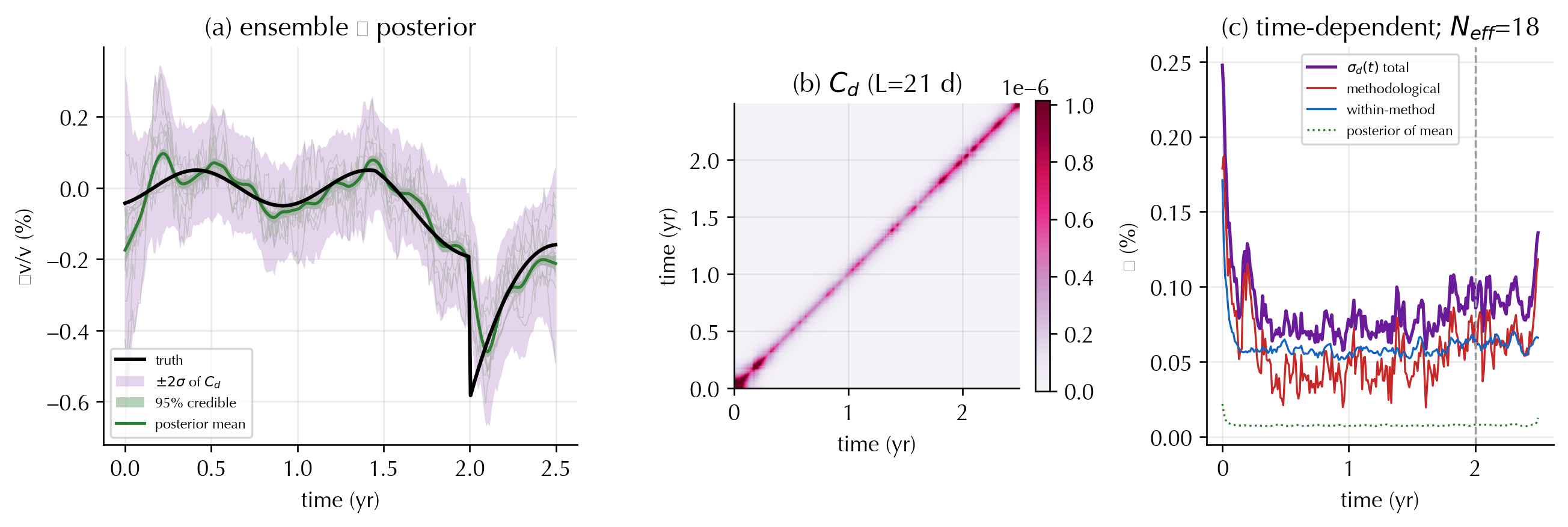
#| fig-cap: "The Bayesian measurement. (a) The ensemble (grey) is marginalised into a posterior mean (purple). Its 95% credible band (estimator precision) is narrow and *under-covers* the truth; the ±2σ band of the marginal data covariance $C_d$ (red) is the honest measurement error and covers it. (b) The time-dependent $C_d$. (c) Its diagonal $σ_d(t)$ split into within-method and methodological parts — wider at the eruption — with the far-tighter posterior-of-the-mean for contrast."
yrs = res.times_days / YEAR_D
sd_cd = np.sqrt(np.diag(res.Cd)); sd_post = np.sqrt(np.diag(res.mu_cov))
fig = plt.figure(figsize=(11, 3.8))
gs = fig.add_gridspec(1, 3, width_ratios=[1.5, 1.0, 1.1])
ax0 = fig.add_subplot(gs[0])
for k in range(run.members.shape[0]):
    ax0.plot(yrs, run.members[k]*100, lw=0.5, color="0.7", alpha=0.6)
ax0.plot(yrs, run.truth*100, color="k", lw=1.8, label="truth", zorder=6)
ax0.fill_between(yrs, (res.mu_mean-2*sd_cd)*100, (res.mu_mean+2*sd_cd)*100,
                 color=C["damage"], alpha=0.18, lw=0, label=r"$\pm2\sigma$ of $C_d$")
ax0.fill_between(yrs, res.mu_lo*100, res.mu_hi*100, color=C["fit"], alpha=0.35, lw=0,
                 label="95% credible")
ax0.plot(yrs, res.mu_mean*100, color=C["fit"], lw=1.5, label="posterior mean")
ax0.set(xlabel="time (yr)", ylabel="δv/v (%)", title="(a) ensemble → posterior")
ax0.legend(fontsize=7, loc="lower left")
ax1 = fig.add_subplot(gs[1])
vmax = float(np.percentile(np.diag(res.Cd), 85))
im = ax1.imshow(res.Cd, cmap="PuRd", origin="lower", vmin=0, vmax=vmax,
                extent=[yrs[0], yrs[-1], yrs[0], yrs[-1]])
ax1.set(title=f"(b) $C_d$ (L={res.corr_length_days:.0f} d)", xlabel="time (yr)", ylabel="time (yr)")
fig.colorbar(im, ax=ax1, fraction=0.046)
ax2 = fig.add_subplot(gs[2])
ax2.plot(yrs, sd_cd*100, color=C["damage"], lw=1.6, label=r"$\sigma_d(t)$ total")
ax2.plot(yrs, res.method_std*100, color=C["thermo"], lw=1.0, label="methodological")
ax2.plot(yrs, res.within_std*100, color=C["hydro"], lw=1.0, label="within-method")
ax2.plot(yrs, sd_post*100, color=C["fit"], lw=1.0, ls=":", label="posterior of mean")
ax2.axvline(2.0, color="0.6", ls="--", lw=1)
ax2.set(xlabel="time (yr)", ylabel="σ (%)", title=f"(c) time-dependent; $N_{{eff}}$={res.n_eff:.0f}")
ax2.legend(fontsize=7)
plt.tight_layout(); plt.show()
```
```{python}
#| label: coverage
tr = run.truth
cred = np.mean((tr >= res.mu_lo) & (tr <= res.mu_hi))
cd95 = np.mean(np.abs(tr - res.mu_mean) <= 2*sd_cd)
print(f"truth inside 95% credible band : {cred:.0%}   (under-covers!)")
print(f"truth within ±2σ of C_d        : {cd95:.0%}   (honest)")
print(f"mean σ: credible {sd_post.mean():.2e}  vs  C_d {sd_cd.mean():.2e}  "
      f"({sd_cd.mean()/sd_post.mean():.0f}× wider)")
```
::: {.callout-important}
The posterior of $\mu$ is the precision of the *combined* estimate; it shrinks
with the ensemble size and **under-covers the truth**, because the pipelines
share a common-mode bias that averaging cannot remove. The object to propagate is
the **marginal measurement covariance**
$$
C_d = D R D + \tau^2\,\mathbf 1\mathbf 1^\top, \qquad
D=\operatorname{diag}\big(\sigma_{\rm tot}(t)\big),\;\; R_{ij}=e^{-|t_i-t_j|/L},
$$ {#eq-cd-bayes}
whose diagonal is time-dependent (wider at the drop and at low coherence), whose
off-diagonal correlation and common-mode term collapse $N_{\rm eff}$ by an order
of magnitude, and which covers the truth at the nominal rate.
:::
## 4. Closing the loop
This is the same $C_d$ the [measurement-UQ page](theory-measurement-uq.qmd)
constructs by hand and the [inference page](theory-uq.qmd) consumes — but here it
is *estimated from the data* by marginalising the processing choice, rather than
assumed. It is the natural input to the GLS stress/depth inversion: supply
`res.Cd` as the data covariance in `codameter.inverse.linear_fit`.
::: {.callout-tip}
## Where this lives in the code
- @eq-bayes, @eq-cd-bayes → `codameter.uq_bayes.gibbs_dvv` / `bayes_dvv_from_ccfs`
- the processing ensemble → `codameter.uq_bayes.run_processing_ensemble`
- the deviation ranking & multiverse that motivate it → `codameter.deviations`
- run the figure standalone → `python -m codameter.uq_bayes`
:::
### References {.unnumbered}
::: {#refs}
:::