---
title: "4 · When decoupling breaks"
subtitle: "Phase 2 — coupling diagnostics and the road to the coupled regime"
jupyter: codameter-pixi
---
::: {.keyidea}
[Step goal]{.k-title}
This is the hinge of the whole arc. Everything so far assumed the stress sources
add **independently**. Phase 2 quantifies *when that assumption fails* — via the
drainage Péclet number and the frequency-dependent $\beta_{\text{eff}}(\omega)$
— and decides whether to trust the linear posterior or escalate to the coupled
inversion. It is [Bayesian model selection](theory-uq.qmd) wearing a fast,
interpretable disguise.
:::
```{python}
#| label: setup
import sys, numpy as np, matplotlib.pyplot as plt
sys.path.insert(0, ".")
from _synth import make_synthetic, build_parkfield_site, set_style, C
from codameter import run_workflow
set_style()
dvv, forcings, eq_times, truth, comp = make_synthetic()
site = build_parkfield_site()
result = run_workflow(dvv, forcings, site, earthquake_times=eq_times)
report = result.phase2.report
```
## The Tier-1 diagnostic
Phase 2 computes the **drainage Péclet number** $\mathrm{Pe}_d$ ([the Péclet number](theory-uq.qmd#eq-peclet)) at
the dominant forcing period, plus the ratio of the effective to drained
acoustoelastic sensitivity from $\beta_{\text{eff}}(\omega)$ ([β_eff(ω)](theory-uq.qmd#eq-betaeff)).
```{python}
#| label: tier1
t1 = report.tier1
print(f"drainage Péclet  Pe_d          : {t1['drainage_peclet']:.1f}")
print(f"β_eff at forcing freq          : {t1['beta_eff_at_forcing']:.1f}")
print(f"β_drained                      : {t1['beta_drained']:.1f}")
print(f"ratio β_eff / β_drained        : {t1['ratio_eff_to_drained']:.4f}")
print(f"escalate?                      : {report.escalate}")
print(f"coupling likelihood            : {report.likelihood['label']}"
      f"  (score {report.likelihood['score']:.2f})")
```
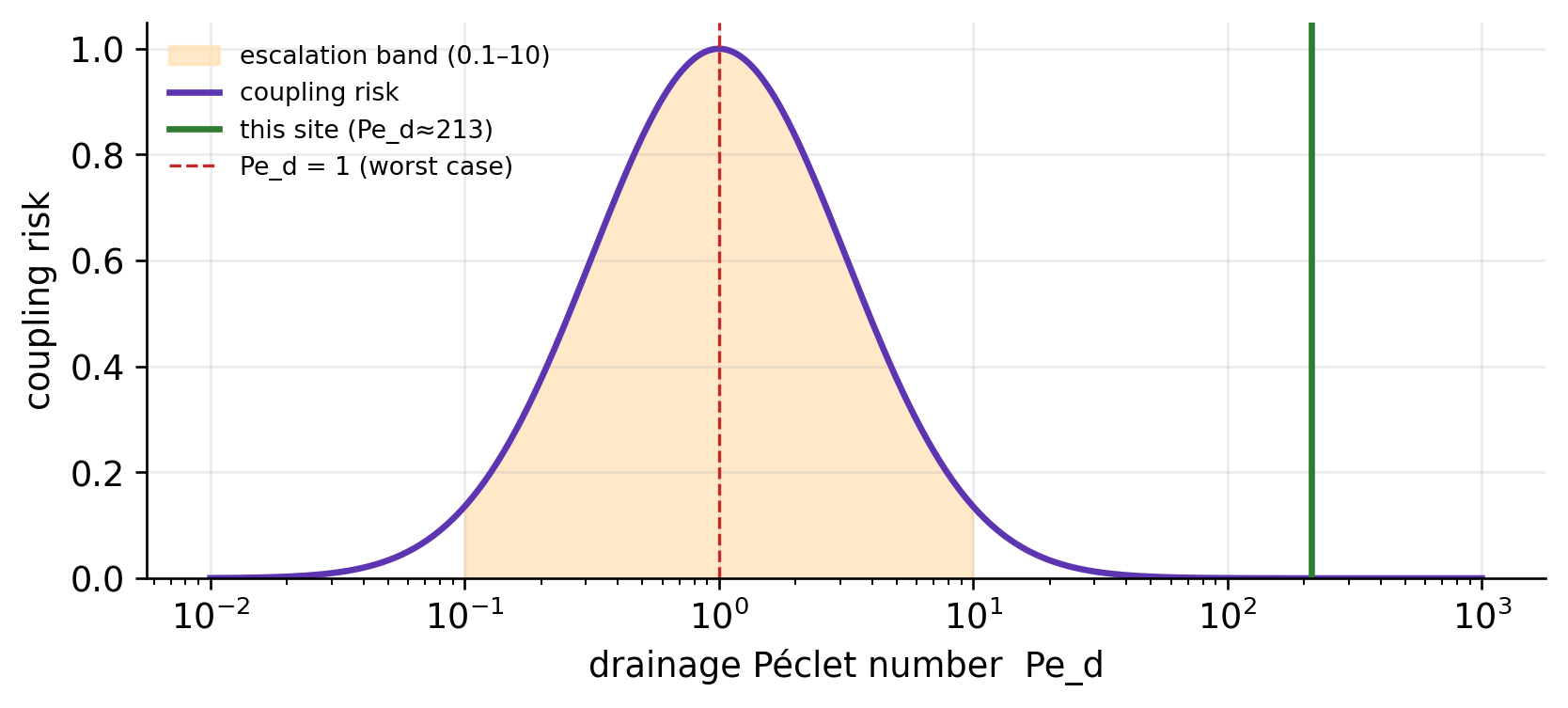
For this synthetic site $\mathrm{Pe}_d \approx 213 \gg 1$: the medium drains
fast relative to the seasonal forcing, $\beta_{\text{eff}}\approx\beta_{\text{drained}}$,
and **decoupling holds**. The linear posterior from
[step 3](tutorial-03-inversion.qmd) is trustworthy. But the interesting science
is what happens as $\mathrm{Pe}_d\to1$.
## The coupling danger zone
The escalation logic is not a hard cliff; it is a smooth risk that **peaks near
$\mathrm{Pe}_d\approx1$**, where the medium can neither fully drain nor stay
undrained over a forcing cycle, and $\beta_{\text{eff}}$ becomes strongly
frequency-dependent and complex. We sweep $\mathrm{Pe}_d$ to draw the map our
site sits on.
```{python}
#| label: fig-danger
#| fig-cap: "The coupling risk surface. Risk (purple) peaks at Pe_d≈1 where drained and undrained responses interfere. Our synthetic Parkfield site (green) sits far in the safe, drained regime — but a clay-rich or deep site can land in the danger zone, where the linear posterior is no longer valid."
pe = np.logspace(-2, 3, 400)
# schematic risk: peaks at Pe=1 on a log axis (matches the package's intent)
risk = np.exp(-0.5 * (np.log10(pe))**2 / 0.5**2)
fig, ax = plt.subplots(figsize=(8, 3.2))
ax.fill_between(pe, 0, risk, where=(pe>=0.1)&(pe<=10), color="#ffe0b2",
                alpha=0.7, label="escalation band (0.1–10)")
ax.plot(pe, risk, color=C["band"], lw=2, label="coupling risk")
ax.axvline(report.tier1["drainage_peclet"], color=C["fit"], lw=2,
           label=f"this site (Pe_d≈{report.tier1['drainage_peclet']:.0f})")
ax.axvline(1.0, color=C["thermo"], ls="--", lw=1, label="Pe_d = 1 (worst case)")
ax.set(xscale="log", xlabel="drainage Péclet number  Pe_d",
       ylabel="coupling risk", ylim=(0, 1.05))
ax.legend(fontsize=8, frameon=False)
plt.show()
```
## Tier scores: a coupling fingerprint
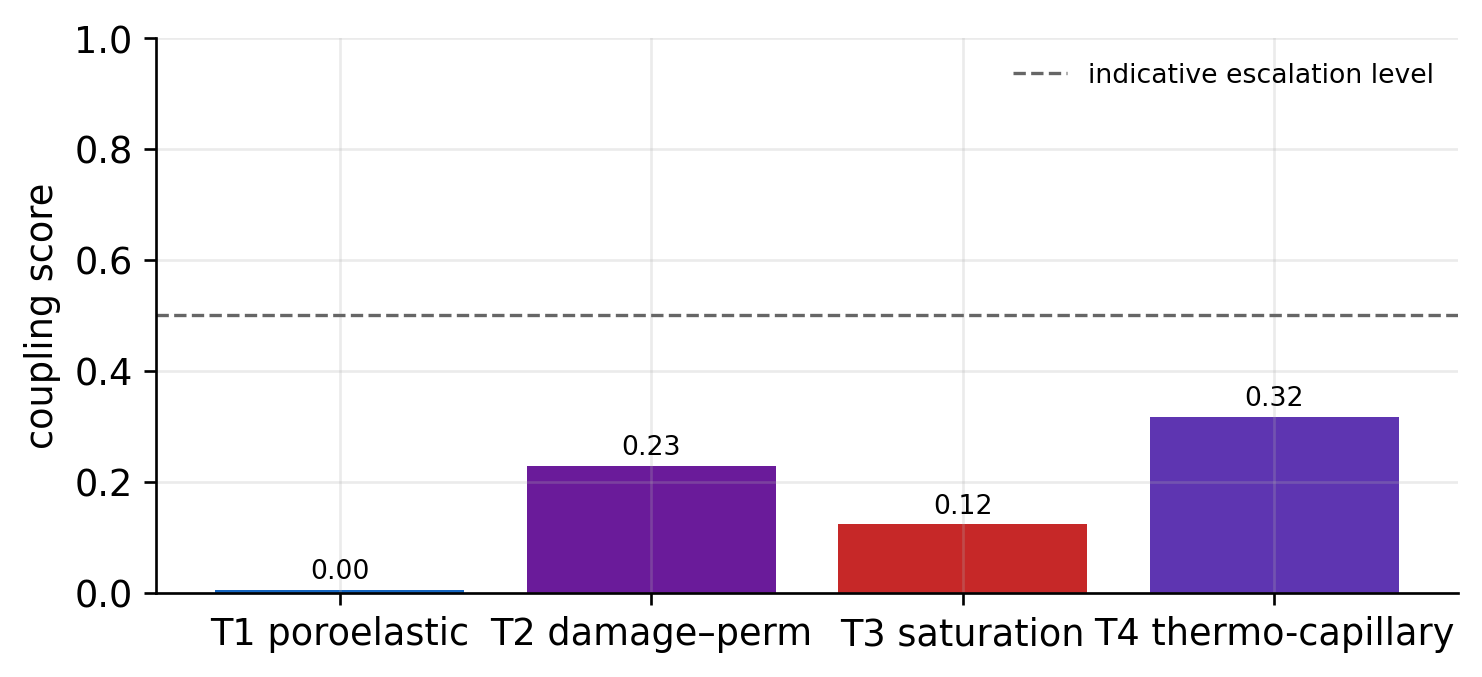
Beyond Tier 1, the report scores four mechanisms (Tiers 2–4 are diagnostic
stubs in v0.1, full models in v0.3): damage–permeability, saturation
nonlinearity, and thermo-capillary coupling. Each returns a normalised score;
together they are a **fingerprint** of how the decoupling might break at this
site.
```{python}
#| label: fig-tiers
#| fig-cap: "Coupling-mechanism scores. Low across the board here — consistent with the safe Pe_d — so the linear model stands. A high bar on any tier would route the workflow toward the coupled inversion of Eq. 19."
ts = report.likelihood["tier_scores"]
labels = {"tier1": "T1 poroelastic", "tier2": "T2 damage–perm",
          "tier3": "T3 saturation", "tier4": "T4 thermo-capillary"}
keys = list(ts.keys())
vals = [ts[k] for k in keys]
fig, ax = plt.subplots(figsize=(7, 3))
bars = ax.bar([labels[k] for k in keys], vals,
              color=[C["hydro"], C["damage"], C["thermo"], C["accent"]])
ax.axhline(0.5, color="0.4", ls="--", lw=1, label="indicative escalation level")
ax.set(ylabel="coupling score", ylim=(0, 1))
ax.legend(fontsize=8, frameon=False)
for b, v in zip(bars, vals):
    ax.text(b.get_x()+b.get_width()/2, v+0.02, f"{v:.2f}",
            ha="center", fontsize=8)
plt.show()
```
## What escalation *means* for uncertainty
::: {.keyidea}
[The decoupled → coupled handoff]{.k-title}
If Phase 2 escalates, the linear-Gaussian posterior of [the Gaussian posterior](theory-uq.qmd#eq-gauss-post) is no
longer the right object: the forward operator becomes **state-dependent**
([the coupled operator](theory-uq.qmd#eq-coupled)), the posterior goes **non-Gaussian**, and we must *sample* it
rather than write it in closed form. The v0.2 `coupled_inversion` backend seeds
an MCMC chain at the WLS solution and draws
$(\beta_{\text{eff}},\mu',c,\tau_{\min},\tau_{\max})$ jointly under the material
priors. Critically, the result is still a `Posterior` object — so
[interpretation](tutorial-05-interpretation.qmd) is **regime-agnostic**.
:::
In v0.1, escalation is surfaced as a clear flag (and `coupled_inversion` raises
an informative `NotImplementedError` with workarounds). The point of this page
is that the decision *to add coupled physics is itself a quantified inference* —
the through-line of the [theory page](theory-uq.qmd).
→ Next: [Interpretation: stress at depth](tutorial-05-interpretation.qmd) —
turning the (here trustworthy) linear posterior into stress, with its
uncertainty.