---
title: "How processing choices move dv/v"
subtitle: "Known truth in, choices applied, artefacts out"
jupyter: codameter-pixi
execute:
warning: false
echo: true
toc: false
---
::: {.keyidea}
[The experiment]{.k-title}
We synthesize a **reference coda** cross-correlation function (CCF), repeat it
over three years while imposing a **known** ground-truth $\delta v/v(t)$, and add
measurement noise. Then we *measure $\delta v/v$ back* under different processing
choices — and, deliberately, some **deviations from best practice**: the wrong
estimator for the signal size, a different way to aggregate a pair's
cross-components, a coda window reused across frequency bands, a moving
reference, a station clock error, seasonal noise in the late coda. Because
the truth is known, **every gap is an artefact of a choice**, not of nature. The
worry is reproducibility: these choices are usually **ad-hoc and undocumented**,
yet they move the answer — so two groups analysing the same data can disagree for
no physical reason. This is the waveform-level companion to the
[best-practice survey](survey-best-practices.qmd) and its
[references](survey-references.qmd).
:::
The machinery lives in
[`codameter.synthetic_demo`](https://github.com/Denolle-Lab/codameter/blob/master/src/codameter/synthetic_demo.py):
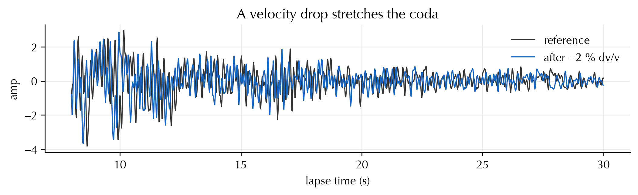
a band-limited, multiply-scattered coda (`make_coda`, and a
frequency-dependent-decay variant `make_freqdep_coda`), a homogeneous velocity
change applied by stretching the coda (`impose_dvv`), daily noisy CCFs
(`daily_ccfs`), artefact injectors (`add_clock_drift`,
`add_seasonal_late_noise`), and the estimators below. A noiseless self-check
confirms recovery to $\sim\!10^{-6}$.
```{python}
#| code-fold: true
#| code-summary: "Set up — imports, style, self-check, and the coda waveform"
import numpy as np
import matplotlib.pyplot as plt
from codameter import synthetic_demo as sd

sd.apply_style()
s = sd.Synth()

truth = np.array([-0.003, 0.0, 0.004])
cur = np.stack([sd.impose_dvv(s.ref, s.t, x) for x in truth])
rec, cc = sd.measure_stretching(cur, s.ref, s.t, band=(0.3, 2.0), fs=s.fs, window=(8, 35))
print("noiseless recovery error:", float(np.max(np.abs(rec - truth))))

cur2 = sd.impose_dvv(s.ref, s.t, -0.02)  # exaggerated −2 % for visibility
fig, ax = plt.subplots(figsize=(8.2, 2.6))
m = (s.t >= 8) & (s.t <= 30)
ax.plot(s.t[m], s.ref[m], color="0.2", lw=1.0, label="reference")
ax.plot(s.t[m], cur2[m], color=sd.C["landslide"], lw=1.0, label="after −2 % dv/v")
ax.set(xlabel="lapse time (s)", ylabel="amp", title="A velocity drop stretches the coda")
ax.legend(loc="upper right"); fig.tight_layout()
```
---
## 1. The full NoisePy / Yuan et al. (2021) estimator suite
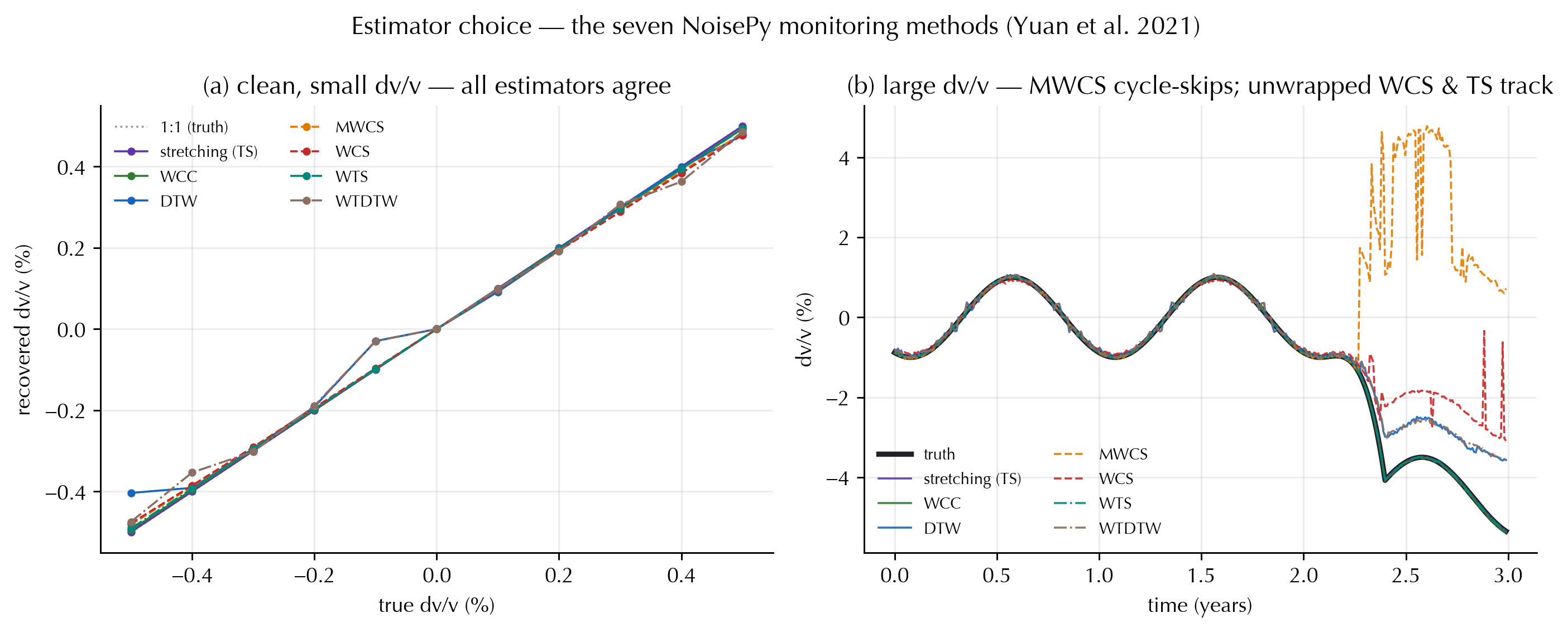
NoisePy's `monitoring_methods` ships **seven** dv/v estimators, and we reproduce
**all seven live** here: `stretching` (TS), `wcc_dvv` (windowed
cross-correlation), `dtw_dvv` (dynamic time warping), `mwcs_dvv` (moving-window
cross-spectrum), and the wavelet-domain `wxs_dvv` (**WCS**, the popular wavelet
cross-spectrum), `wts_dvv` (wavelet stretching), and `wtdtw_dvv` (wavelet DTW).
**@Yuan2021** benchmark the suite numerically.
On **small, clean** $\delta v/v$ they all sit on the 1:1 line (panel a) — so the
*choice does not matter and the result is reproducible*. The choice bites at
**large** $\delta v/v$ (panel b), where the methods split by **family**:
- **Stretching family** (TS, WTS) — and WCC — match the whole dilated coda and
stay accurate;
- **Phase methods** read delays from a wrapped phase. **MWCS** wraps at half a
period and **cycle-skips**; **WCS** *would* too, but here it **unwraps the phase
in 2-D** [@Mao2020] — so the very same family succeeds or fails purely on
the **unwrapping choice**;
- **Warping methods** (DTW, WTDTW) track but **under-shoot** the largest strains
(a discretized-warp bias).
No method is simply "right"; the point is that an **ad-hoc estimator choice** —
or even a sub-choice like whether to unwrap — silently changes the answer once
the signal leaves the small-amplitude regime.
```{python}
#| code-fold: true
sd.fig_methods();
```
---
## 2. Aggregating cross-components
A single station pair carries several cross-component CCFs (ZZ, ZN, …), each a
noisy view of the *same* $\delta v/v$. How you combine them is a workflow choice
that is almost never reported, yet it changes both the value **and the
uncertainty**:
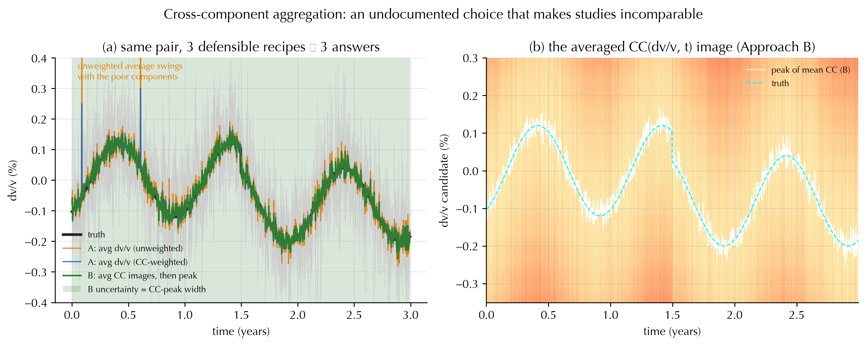
- **A — average the dv/v.** Peak-pick each component's stretching curve
$\mathrm{CC}(\varepsilon, t)$, then **average the per-component dv/v**. Its
uncertainty is the *ensemble spread* of the picks. *Unweighted*, a few poor
components drag the mean around; **CC-weighted**, they are suppressed.
- **B — average the images.** Stack the $\mathrm{CC}(\varepsilon, t)$ images
across components **first**, then peak-pick once. Its uncertainty is the *width
of the averaged CC peak* — a different statistical object entirely.
All three are reasonable and appear in the literature (including NoisePy). On the
same station pair they give visibly different time series — A-unweighted swings
with the poor components while CC-weighted-A and image-stack-B track — and they
propagate uncertainty along **incompatible pathways**, so two studies using
different recipes are simply not comparable.
```{python}
#| code-fold: true
sd.fig_aggregation();
```
---
## 3. Station-pair aggregation and the error bar you report
Add the next layer up — many station pairs, each already a coherence-weighted
average over its cross-components, combined into a **network** $\delta v/v(t)$.
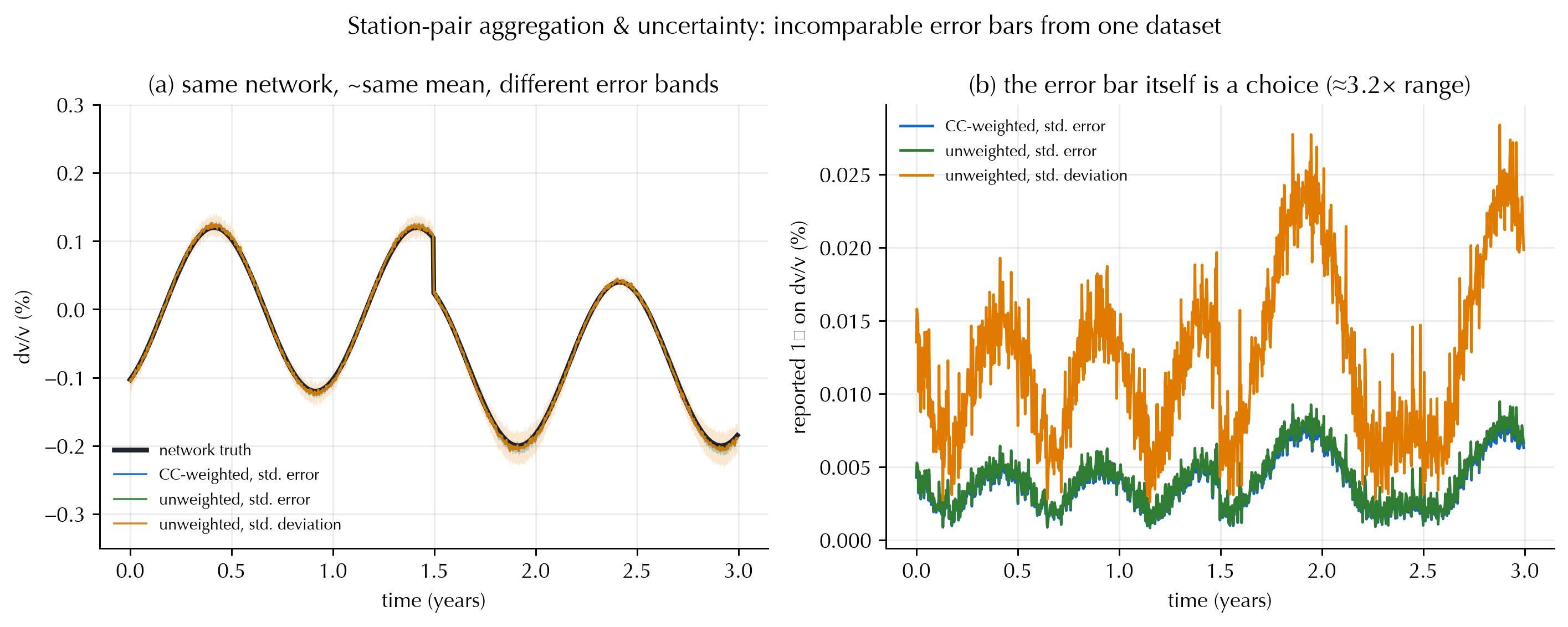
Now the choice is how to summarize the *uncertainty*, and three conventions all
appear in the literature:
- **CC-weighted standard error** — weight pairs by coherence, $\sigma =
\sigma_w/\sqrt{N_\mathrm{eff}}$;
- **unweighted standard error** — $\sigma = \mathrm{std}/\sqrt{N}$;
- **standard deviation** — report the between-pair *scatter*, not divided by
$\sqrt{N}$.
On the same network the **means nearly coincide**, but the reported $1\sigma$
spans a factor of $\sim\!\sqrt{N}$ (panel b). A velocity change that is "$3\sigma$
significant" under the tight convention is "$1\sigma$, not significant" under the
conservative one — from the *same data*. Error bars are not comparable across
studies unless the aggregation and the SE-vs-SD convention are both stated.
```{python}
#| code-fold: true
sd.fig_uncertainty();
```
---
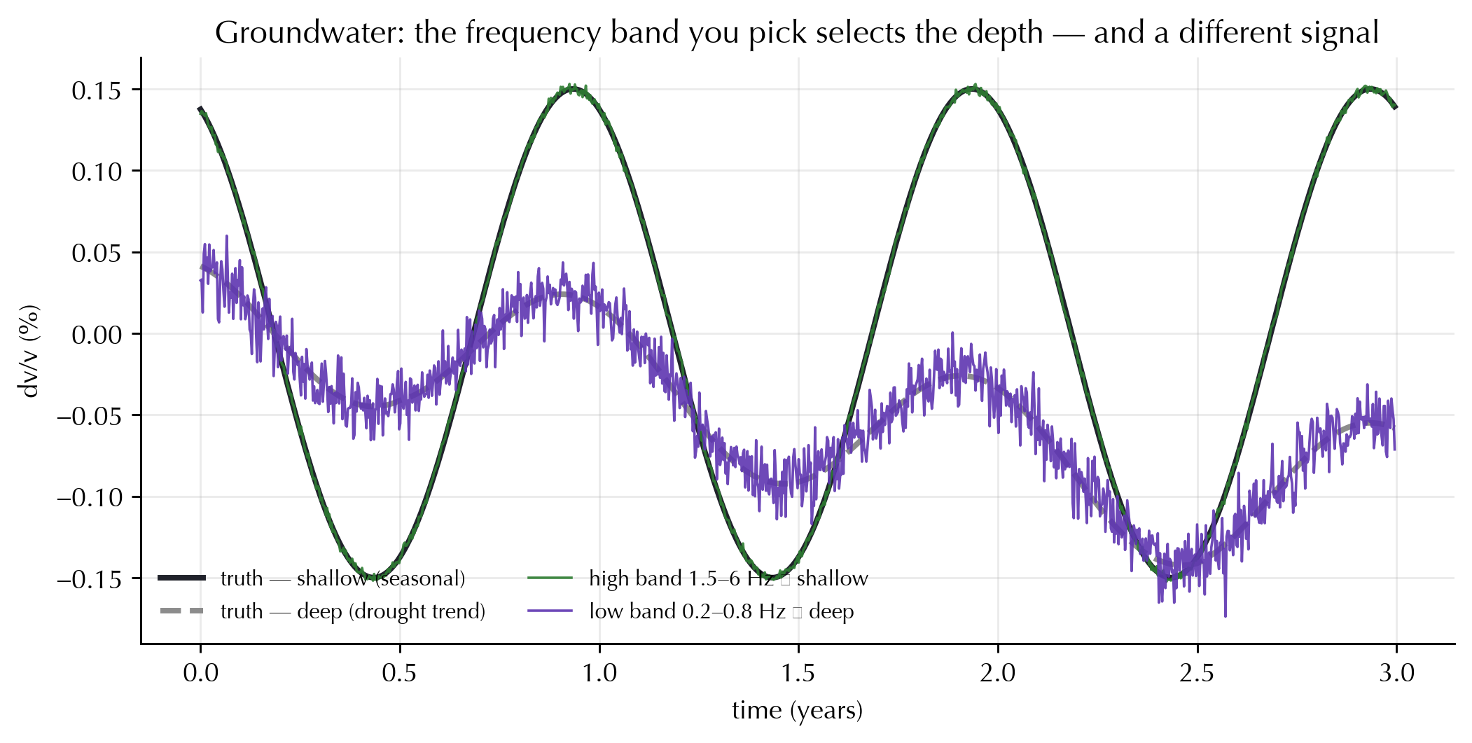
## 4. Frequency band selects the depth and the signal
Give the medium **two layers**: a shallow one with a strong seasonal cycle and a
deep one with a multi-year drought trend, each living in a different part of the
coda spectrum. Band high → you recover the shallow seasonal signal; band low →
the deep trend. **The band is not a free knob — it chooses what you measure**
(survey rule 6).
```{python}
#| code-fold: true
sd.fig_frequency_depth();
```
---
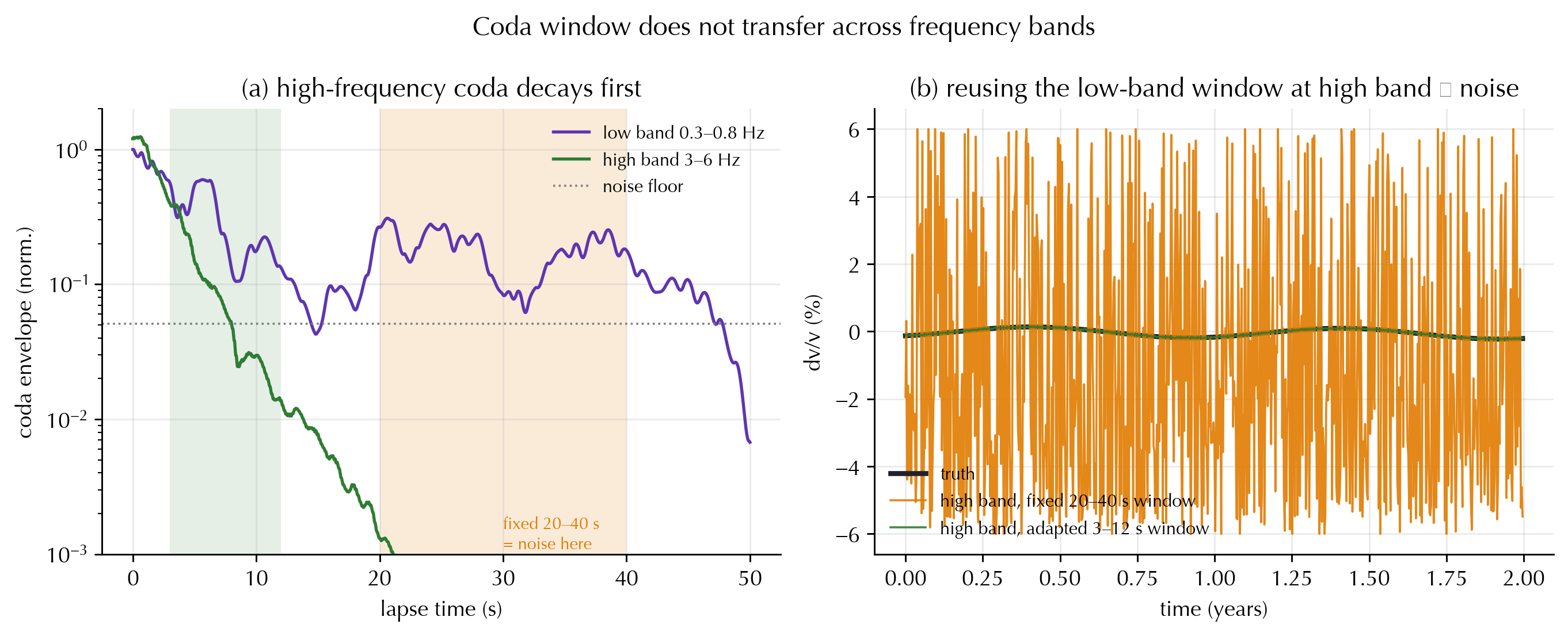
## 5. The coda window does not transfer across bands
A common deviation: pick one lapse window (say 20–40 s) and reuse it at every
frequency. But the coda **decays faster at high frequency** ($A(t)\propto
e^{-\pi f t/Q_c}$), so a window that is full of signal at low frequency is **pure
noise** at high frequency (panel a). Measuring the high band in that fixed late
window returns garbage; an earlier, SNR-matched window recovers the truth (panel
b). The window must scale with the band — ideally set from the coda envelope / a
fixed number of mean-free-times, not copied across bands.
```{python}
#| code-fold: true
sd.fig_window_band();
```
---
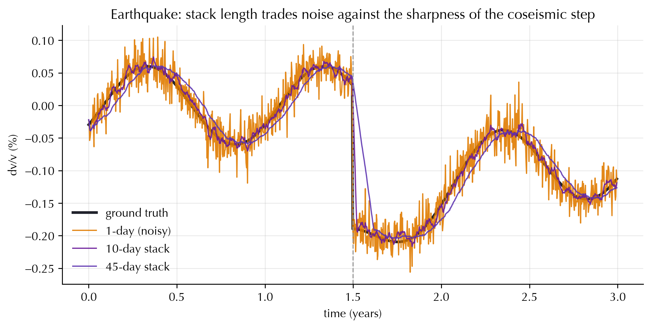
## 6. Stacking length trades resolution against noise
A coseismic **step** under a seasonal cycle. A 1-day CCF is noisy but captures
the step's timing; a long trailing stack suppresses noise but **rounds off and
delays the step** — the resolution/precision trade-off behind stacking choices
(survey rule 7).
```{python}
#| code-fold: true
sd.fig_stacking();
```
---
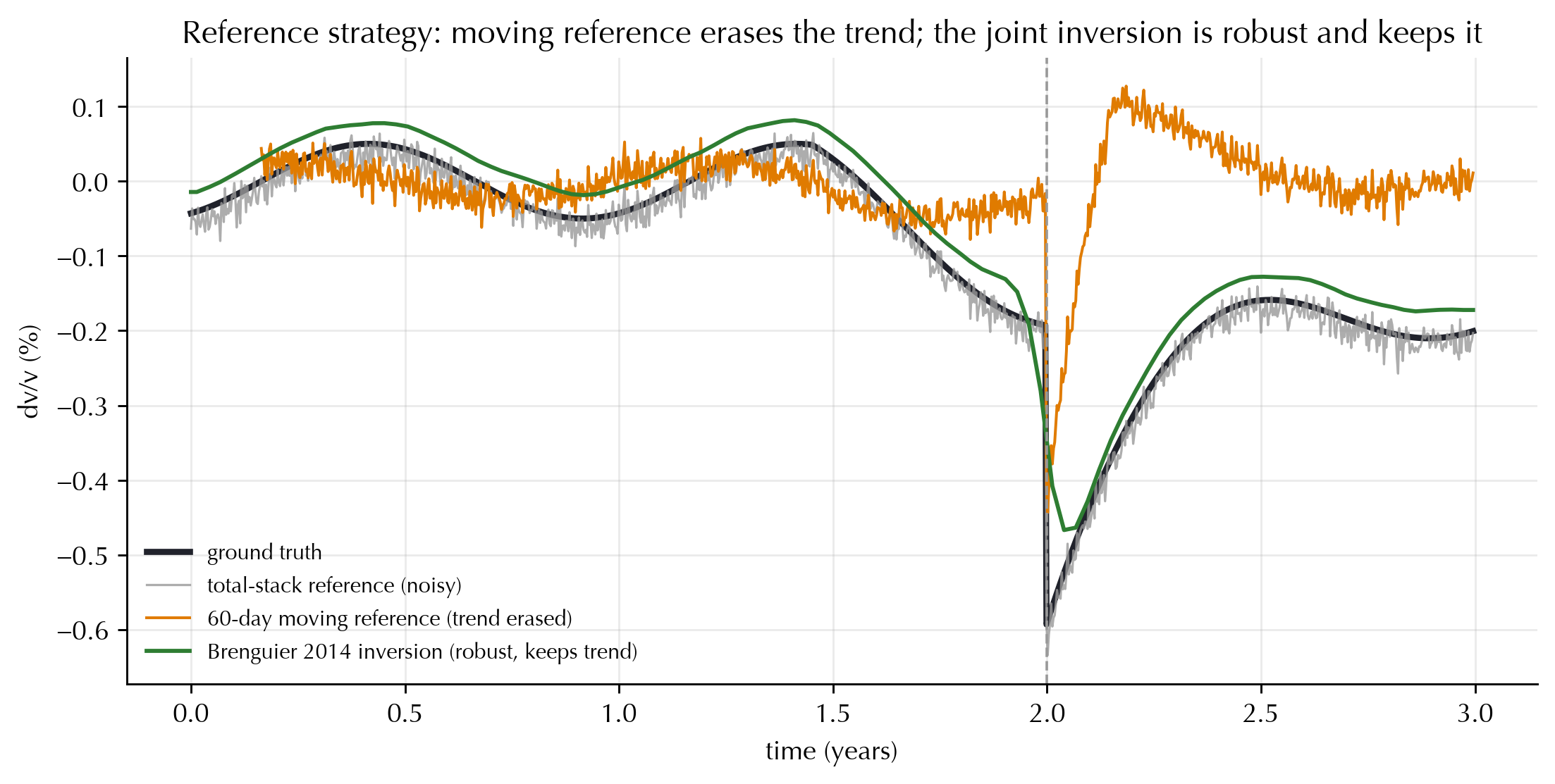
## 7. Reference strategy
How you define the reference sets what survives. A **total-stack** reference is
unbiased but noisy; a **moving** reference re-baselines continuously and so
**erases slow trends** (the pre-eruptive decline vanishes); the **Brenguier et
al. (2014) joint inversion** measures relative $\delta v/v$ between many short
stacks and inverts ``x_i − x_j = m_{ij}`` with a smoothness penalty — robust to
any single reference *and* trend-preserving.
```{python}
#| code-fold: true
sd.fig_reference();
```
---
## 8. Deviations that *manufacture* dv/v
Not every wiggle is a velocity change. Two classic instrument/environment
artefacts inject **spurious** $\delta v/v$:
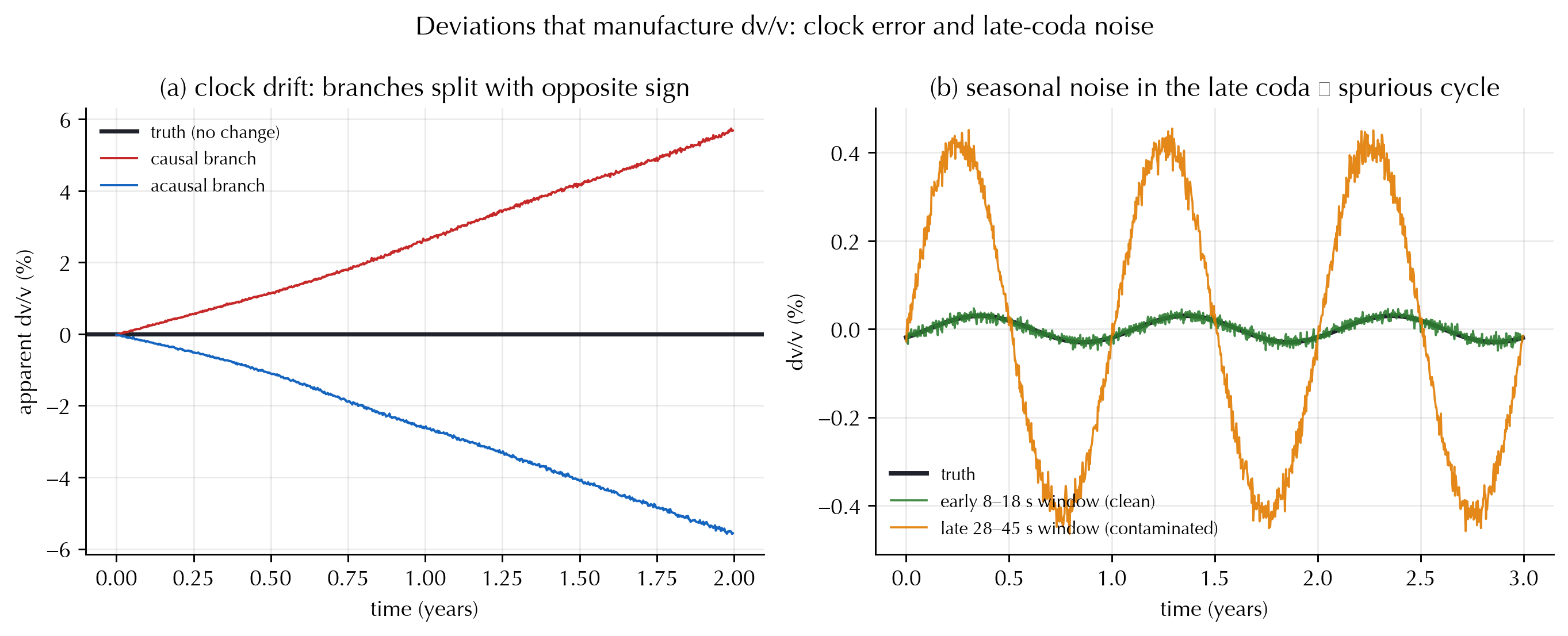
- **Station clock error** (panel a). A timing drift delays the whole CCF — a
*constant* lag, independent of lapse — so it appears with **opposite sign on
the causal and acausal branches**. A real velocity change moves both the same
way, so measuring the two branches separately is the diagnostic.
- **Seasonal noise in the late coda** (panel b). A seasonally changing
noise-source distribution warps the low-SNR late coda, so a **late** window
reports a coherent spurious *seasonal* $\delta v/v$ many times the real signal,
while an **early**, higher-SNR window stays clean (the [@Zhan2013; @Daskalakis2016] warning).
```{python}
#| code-fold: true
sd.fig_artifacts();
```
---
## 9. The garden of forking paths
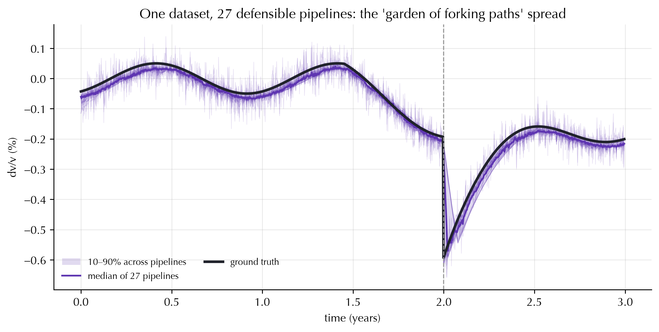
Finally, take one volcano dataset and run **27 individually reasonable pipelines**
(3 bands × 3 windows × 3 stack lengths) with a common pre-eruption reference. The
median tracks the truth, but the 10–90 % spread across pipelines fans out **most
where it matters** — at the sharp co-eruptive drop. The honest object is a
*distribution* of $\delta v/v$ over processing choices, which is exactly what
[`codameter.uq_processing`](https://github.com/Denolle-Lab/codameter/blob/master/src/codameter/uq_processing.py)
samples and marginalizes.
```{python}
#| code-fold: true
sd.fig_multiverse();
```
---
## Takeaways
| Choice / deviation | Shown with | Consequence of deviating |
| --- | --- | --- |
| Estimator — all 7 NoisePy methods | @Yuan2021 suite | At large dv/v: MWCS cycle-skips, 2-D-unwrapped WCS recovers, warps (DTW, WTDTW) under-shoot |
| Cross-component aggregation | Station pair, 6 components | Avg-dv/v vs avg-CC-images, weighted vs not → different value *and* uncertainty |
| Station-pair aggregation & σ | 9-pair network | Same mean, but reported 1σ differs ~√N (SE vs SD, weighted vs not) |
| Frequency band | Groundwater 2-layer | Band selects depth → a *different* signal |
| Coda window vs band | Frequency-dependent coda | A fixed late window is pure noise at high frequency |
| Stack length | Earthquake step | Long stack smears and delays the step |
| Reference scheme | Volcano | Moving reference erases the trend; joint inversion is robust |
| Clock error | Stable medium | Spurious dv/v, opposite-sign on causal vs acausal branches |
| Seasonal late-coda noise | Stable medium | Spurious *seasonal* dv/v from a late window |
| All of the above | Multiverse | Spread across pipelines ≈ size of the signal |
The constructive response is the survey's
[cross-cutting rules](survey-best-practices.qmd#cross-cutting-methodology-rules):
quantify the within-choice error, scale the band/window to the target depth, fix
the reference deliberately, check the causal/acausal branches for timing errors,
weight by SNR, and — when in doubt — **sample the choices and report the
marginal**.
*Reproduce locally:* `pixi run python literature/synthetic_dvv_demo.py`.
### References {.unnumbered}
::: {#refs}
:::