---
title: "3 · Linear superposition & inversion"
subtitle: "Phases 3–4 — the closed-form Gaussian posterior in action"
jupyter: codameter-pixi
---
::: {.keyidea}
[Step goal]{.k-title}
Build the design matrix $X$ from the decoupled forward models, then solve the
weighted least-squares problem to get the **full Gaussian posterior**
$\mathcal{N}(\hat m,\hat C)$ of [the Gaussian posterior](theory-uq.qmd#eq-gauss-post) — not just the best-fit
amplitudes, but their covariance, which is what makes the downstream stress
uncertainty honest.
:::
```{python}
#| label: setup
import sys, numpy as np, matplotlib.pyplot as plt
sys.path.insert(0, ".")
from _synth import make_synthetic, build_parkfield_site, set_style, C
from codameter import run_workflow
set_style()
dvv, forcings, eq_times, truth, comp = make_synthetic()
site = build_parkfield_site()
result = run_workflow(dvv, forcings, site, earthquake_times=eq_times)
fit = result.phase4.fit
```
## Phase 3 — the design matrix
Each enabled forcing contributes one column to $X$. The columns are the
footprints from [step 2](tutorial-02-forward.qmd), now assembled as *predictors*
whose amplitudes are unknown.
```{python}
#| label: design
pm = fit.predictor_matrix
print("parameters :", fit.parameter_names)
print("design X   :", pm.X.shape, "(n_obs × n_par)")
```
## Phase 4 — weighted least squares → posterior
The fit minimises the weighted misfit of [the weighted misfit](theory-uq.qmd#eq-loglike). Because the model is
linear and the noise Gaussian, the result is an *exact* multivariate-normal
posterior over the amplitudes. `fit.summary()` is the tidy view; `fit.posterior`
is the object the rest of the pipeline propagates.
```{python}
#| label: summary
fit.summary()
```
```{python}
#| label: gof
print(f"reduced χ² : {fit.chi2_reduced:.3f}   (≈1 ⇒ residuals consistent with σ)")
print(f"rank       : {fit.rank} / {fit.n_par}")
```
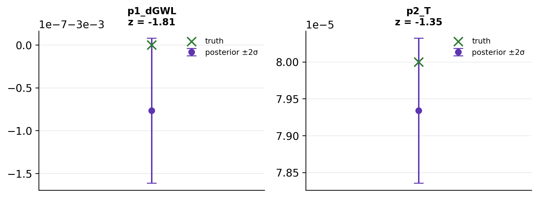
## Did we recover the truth?
Because this is synthetic, we know the amplitudes that built the data. The
posterior should bracket them. We plot each fitted amplitude with its
$\pm2\sigma$ interval against the (known) truth.
```{python}
#| label: fig-recovery
#| fig-cap: "Parameter recovery. Fitted posterior means (points) with ±2σ bars bracket the synthetic truth (crosses) for the two physically interpretable amplitudes. The intervals come straight from the diagonal of Ĉ."
post = fit.posterior
names = ["p1_dGWL", "p2_T"]
truth_map = {"p1_dGWL": truth["p1_dGWL"], "p2_T": truth["p2_T"]}
fig, axes = plt.subplots(1, 2, figsize=(8, 3))
for ax, nm in zip(axes, names):
    m, s = post.marginal(nm)
    ax.errorbar([0], [m], yerr=[2*s], fmt="o", color=C["band"], capsize=5,
                label="posterior ±2σ")
    ax.scatter([0], [truth_map[nm]], marker="x", s=90, color=C["fit"],
               zorder=5, label="truth")
    z = (m - truth_map[nm]) / s
    ax.set_title(f"{nm}\nz = {z:+.2f}", fontsize=10)
    ax.set_xticks([]); ax.legend(fontsize=8, frameon=False)
plt.tight_layout(); plt.show()
```
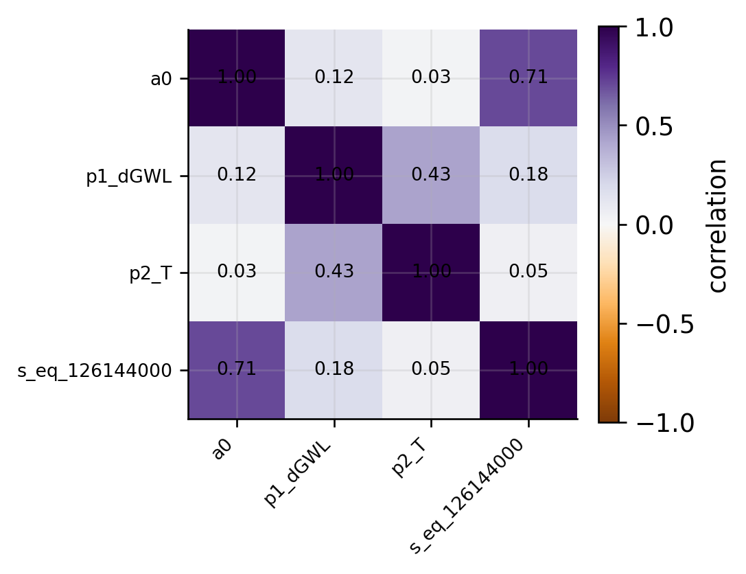
## The covariance is the point
A point estimate would stop at the means. But the parameters are **correlated**
— the thermoelastic and hydrological amplitudes trade off because both carry a
seasonal cycle — and ignoring that correlation underestimates the stress
uncertainty in [step 5](tutorial-05-interpretation.qmd). Here is the posterior
correlation matrix straight from $\hat C$.
```{python}
#| label: fig-corr
#| fig-cap: "Posterior correlation matrix from Ĉ. Off-diagonal structure is the trade-off between forcings that a single-number report discards. Propagating it is exactly the delta-method step ∇gᵀ Ĉ ∇g of the theory page."
cov = post.cov
d = np.sqrt(np.diag(cov))
corr = cov / np.outer(d, d)
fig, ax = plt.subplots(figsize=(4.6, 4))
im = ax.imshow(corr, vmin=-1, vmax=1, cmap="PuOr")
ax.set_xticks(range(len(post.parameter_names)))
ax.set_yticks(range(len(post.parameter_names)))
ax.set_xticklabels(post.parameter_names, rotation=45, ha="right", fontsize=8)
ax.set_yticklabels(post.parameter_names, fontsize=8)
for i in range(len(corr)):
    for j in range(len(corr)):
        ax.text(j, i, f"{corr[i,j]:.2f}", ha="center", va="center",
                fontsize=8, color="k")
fig.colorbar(im, ax=ax, fraction=0.046, label="correlation")
plt.tight_layout(); plt.show()
```
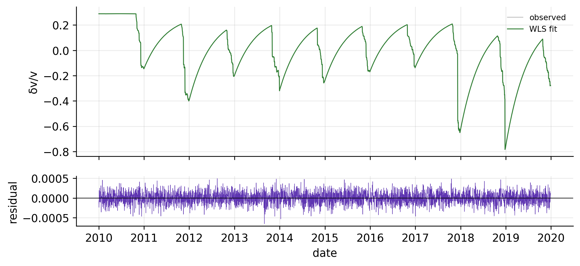
## The fit and its residuals
```{python}
#| label: fig-fit
#| fig-cap: "Top: observed vs fitted δv/v. Bottom: residuals. Whether these residuals are white noise — or hide structure betraying a broken decoupling assumption — is the question Phase 5 and the coupling diagnostics answer next."
fitted = fit.fitted
resid = fit.residuals
fig, axes = plt.subplots(2, 1, figsize=(9, 4), sharex=True,
                         gridspec_kw={"height_ratios": [3, 1]})
axes[0].plot(dvv.index, dvv.dvv, color="0.6", lw=0.5, label="observed")
axes[0].plot(dvv.index, fitted, color=C["fit"], lw=0.9, label="WLS fit")
axes[0].set(ylabel="δv/v"); axes[0].legend(fontsize=8, frameon=False)
axes[1].plot(dvv.index, resid, color=C["accent"], lw=0.4)
axes[1].axhline(0, color="k", lw=0.6)
axes[1].set(ylabel="residual", xlabel="date")
plt.show()
```
→ Next: [When decoupling breaks](tutorial-04-coupling.qmd) — the diagnostics
that decide whether this linear posterior is trustworthy.