01 / CRITICAL ZONE
Which shallow layer changed?
A 10–18 Hz weathered-column experiment: rainfall-like softening, a competing shallow oscillation, and depth resolution with correlated frequency errors.
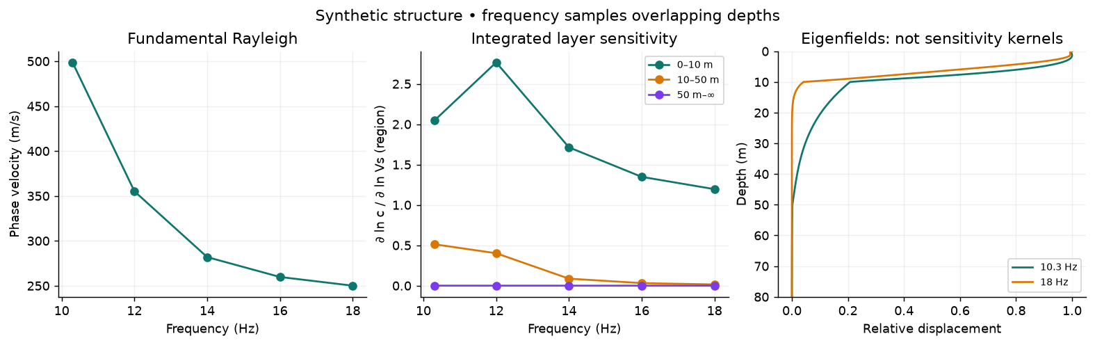
Work through the questions behind a velocity-change curve: which depths are sampled, which changes can be distinguished, and how water and acquisition geometry affect the inference.
Five executed notebooks • 18 computed figures • synthetic experiments at field scales
Read the rendered results or download an executable notebook.
A 10–18 Hz weathered-column experiment: rainfall-like softening, a competing shallow oscillation, and depth resolution with correlated frequency errors.
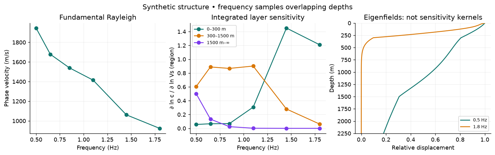
Compare elastic-change hypotheses in a basaltic edifice. Inspect frequency coverage, averaging matrices, and posterior depth tradeoffs before assigning a process.
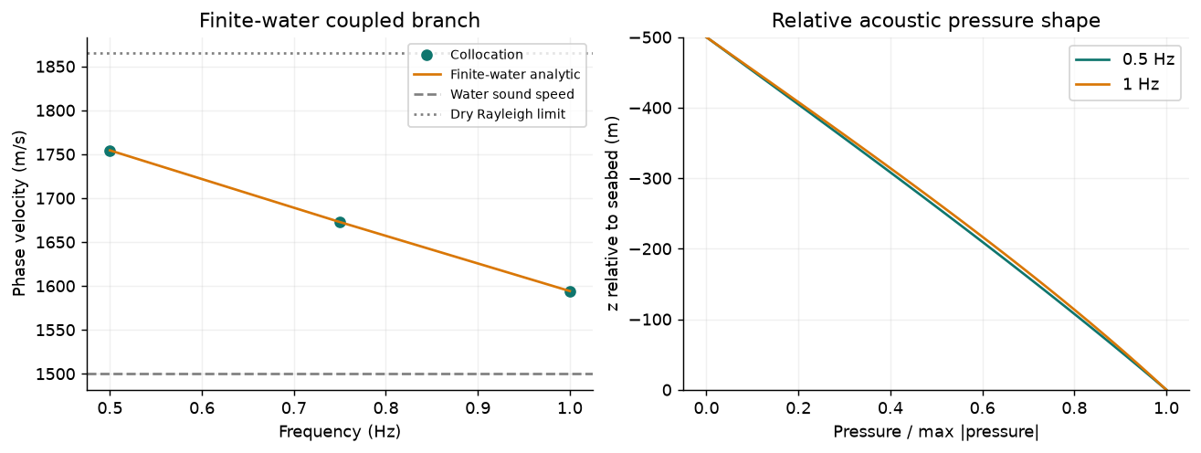
Verify a finite-water coupled branch against an analytical secular equation, then carry water-column uncertainty into seabed velocity-change inference.
Compare joint path–depth inference with a two-stage phase-map inversion. They agree when the full covariance is retained in this linear acquisition experiment.
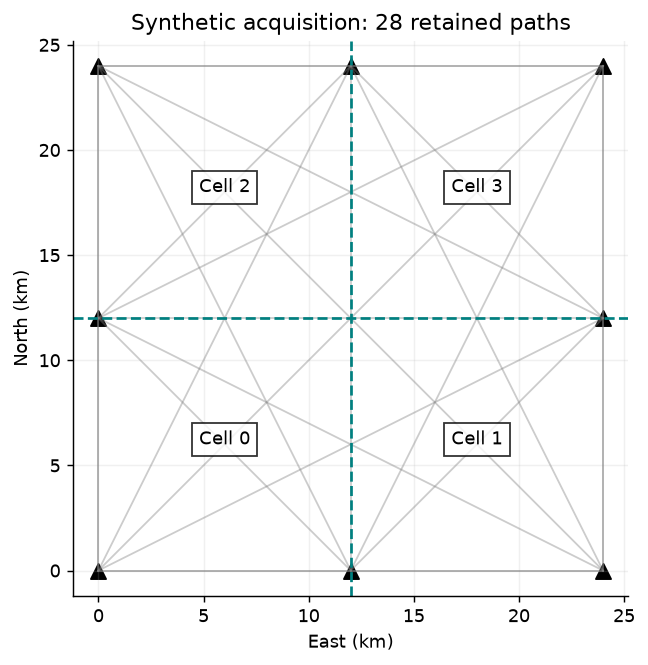
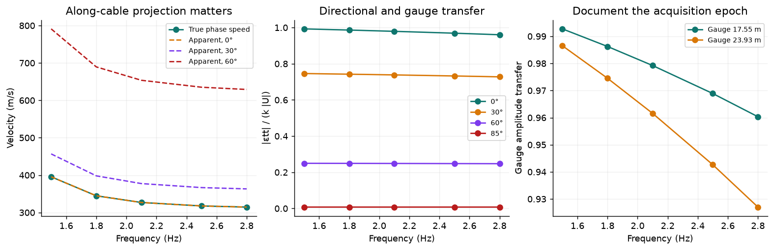
Published KKFL-S acquisition parameters meet a synthetic layered seabed. Correct along-cable projection, examine gauge response, fit absolute dispersion, then invert small seabed changes with water uncertainty.
Field acquisition facts are cited. The seabed geology and dispersion picks are explicitly synthetic.
Define the observableThe monitoring operator models direct fundamental-mode phase changes. Coda stretching and MWCS require an additional estimator-specific sensitivity model.
Ask about resolutionLayer sensitivities overlap. Good data fit does not establish a uniquely localized depth change. Examine uncertainty, averaging, and alternative backgrounds.
Separate elasticity from causeTemperature, effective stress, damage, and fluid effects may yield similar elastic changes. Interpretation needs environmental or volcanic observations.
Each notebook is rerun from a fresh kernel before publication; assertions gate deployment. These are small elastic reference calculations, conditional on the stated models and priors. Local execution instructions · Machine-readable execution report